Analysis Of Variance
Analysis of variance (ANOVA) is an inferential statistics technique that involves a statistical test for the significance of differences between mean scores of at least two groups across one or more than one variable. ANOVA can be used to test for statistical significance using categorical independent variables in conjunction with a continuous dependent variable. ANOVA is based on the comparison of variance between groups with variance within groups, emerging as the F ratio, or F statistic.
ONE-WAY ANOVA
We will perform an ANOVA test using “RACE” as the independent variable and respondent’s income as the dependent variable. To measure race/ethnicity, we will use the recoded, four-category version of that variable. (For details on how to recode “RACE,” , “Transforming Variables.”) For income, we could use “REALRINC,” but suppose it were not available and all we had to work with was “RINCOM16,” a collection of ordered, mutually exclusive, and exhaustive income ranges. We will need to recode “RINCOM16” because it is measured by numeric categories corresponding to nonequivalent ranges of annual earnings. We can use the midpoint dollar amount of each of those ranges to approximate income for respondents in each category. To make it so, follow these instructions:
Transform → Recode into Different Variables . . .
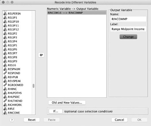
In the “Recode into Different Variables” dialog box, select “RINCOM06” and move it from the variable bank on the left over to the area for “Numeric Variable → Output Variable.” Now, type a new name in the “Output Variable” area, and also a descriptive label. Next, click the “Change” button, and make sure the change was recorded in the “Numeric Variable → Output Variable” listing.
At this point, click the “Old and New Values . . .” button, and you will be presented with the following dialog box:
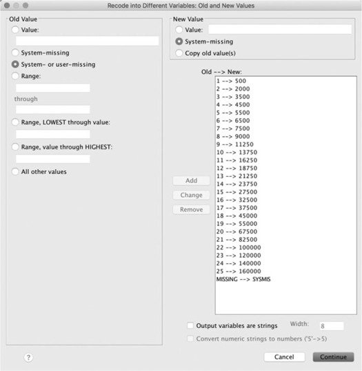
In the “Recode into Different Variables: Old and New Values” dialog box, you will enter the numeric values from the original variable and the corresponding midpoint of each of those ranges as the new values. Don’t forget to maintain missing cases properly. The numeric scores on “RINCOM06” and the appropriate midpoints are displayed in the image on page 158. Note that for category 25, a true midpoint could not be constructed.
In the preceding example, the midpoint of each interval is used as an estimate; there are, however, other methods for estimating such intervals. Once you click “Continue” and then “OK” in the prior window, SPSS Statistics will create your newly coded variable, “RINCOMMP”: respondent’s income range midpoint estimate.
Now, to carry out the one-way ANOVA test, use the following menus:
Analyze → Compare Means → One-Way ANOVA . . .
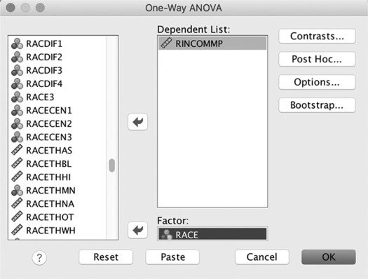
In the dialog box that is presented, choose the dependent and independent (factor) variables for your analysis. Click the “Options . . .” button to customize your selections further; this will bring up the following dialog box:
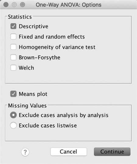
Here, descriptive statistics have been requested as well as a plot of the means. Cases have been excluded analysis by analysis. After clicking “Continue” here and then “OK” in the “One-Way ANOVA” window, SPSS Statistics will run the test. The output that follows begins with the descriptive statistic information and is followed by the ANOVA results:


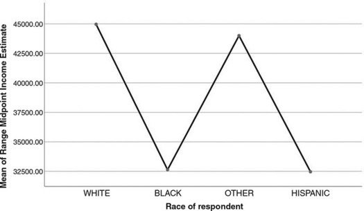
The F statistic has been calculated at 16.529 with 3 degrees of freedom. In this example, F is significant at the p = .000 level. The means plot has also been provided by SPSS Statistics as requested and has been reproduced on page 161. Although the line itself may not be of much use here, as perhaps it might be in the case of an ordinal variable, it is easy to quickly ascertain the differences in the means from this graph.
ANOVA IN REGRESSION
To examine ANOVA in an ordinary least squares regression model, use the following menus:
Analyze → Regression → Linear . . .
:
Analyze → Regression → Linear . . .
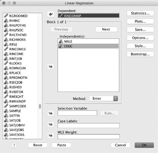
When presented with the “Linear Regression” dialog box, enter your dependent variable and independent variables. To obtain additional partial correlation values or estimates, click the “Statistics . . .” button and mark the appropriate boxes in that dialog box.
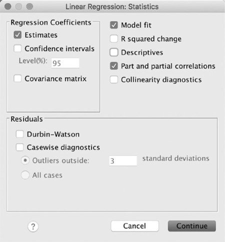
After you click “Continue” in the above dialog box and then “OK” in the “Linear Regression” dialog box, the following output will be presented. Note that the sum of squares and mean squares have been provided, as well as the F statistic and its p value (indicating whether it is statistically significant).
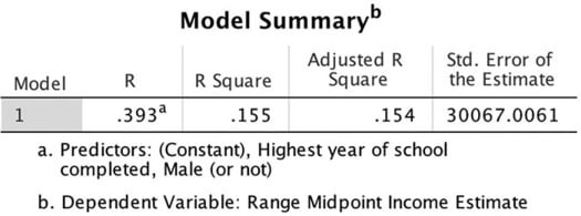
Remember that r-square is a proportional reduction in error statistic, and when r 2 = .155, we can interpret that to mean that 15.5% of the variation in income is explained by variation in both education and gender.
In the following, you can see that F was calculated at 144.28 with 2 degrees of freedom. This value is statistically significant at p = .000.

As part of the linear regression command, SPSS Statistics also provides the regression model coefficient output, printed below. Notice that, on average, men are predicted to make almost $15,000 per year more than women, and each additional year of education is estimated to bring an average of just under $4,000 per year in annual earnings, not controlling for any other factors.


Access the full 2016 data file and the 1972–2016 Cumulative Codebook at the student study site: study.sagepub.com/wagner7e.
Descriptions of Images and Figures
In this window, a long list of values is present in a column on the left side. The values are RELSP 1, RELSP 2, RESPNUM, RGROOMED, RINCOME, and so on.
To the right of the list is a box titled “Numeric Variable, a right arrow. Output Variable:” this box shows the value:
- RINCOME16, a right arrow, RINCOMMP.
- There is a left arrow next to this box to include values from this box to the list on the left.
To the right of this box is a section named Output Variable.
- Name. Below is a bar that shows the value “RINCOMMP”
- Label: below is a bar that shows the value
- The button “Change” is below this.
End section.
A button named “Old and New Values”
A section with the button “If” and the text “Optional Case Selection Condition”. End section.
There are four buttons at the bottom of the window:
- A question mark
- Reset
- Paste
- Cancel
- OK.
In this window, on the left side, there is a section named Old Value. It shows the following data:
- Check circle: Value. There is a bar below this.
- Check circle: System-missing
- Check circle: System- or user-missing. This option is selected
- Check circle: Range. There is a bar below this.
- Through: There is a bar below this.
- Check circle: Range, LOWEST through value: There is a bar below this.
- Check circle: Range, value through Highest: There is a bar below this.
- Check circle: All other values.
End section
On the right side, at the top in the window, there is a section named New Value:
- Check circle: Value. There is a bar next to this.
- Check circle: System-missing. This option is selected
- Check circle: Copy old value or values
End section
Below this is a long table titled “Old, right arrow New” it shows the values 1 to 500, 2 to 2000, and so on till 25 to 160000 and MISSING to SYSMIS. There are the buttons Add, Change, and Remove next to this table.
Below the table are the following:
- A checkbox: Output variables are strings. Width: value 8 in a box.
- A checkbox: Convert numeric strings to numbers; “5” to “5.”
At the bottom of the window are the following buttons:
- Cancel
- Continue.
In this window, there is a list of variables on the left such as RACDIF1, RACE3, RACECEN1, RACETHWT, and so on.
To the right of this table is a list named “Dependent List:”. This shows the value RINCOMMP, which is selected. There is a left arrow next to this list, to include values from this list to the list on the left.
Below the Dependent list is “Factor”. This shows the value “RACE”. There is a left arrow next to this to include values from this list to the list on the left.
To the right of the dependent list are the following buttons:
- Contrasts
- Post Hoc
- Options
- Bootstrap
At the bottom of the window are the following buttons:
- Question mark
- Reset
- Paste
- Cancel
- OK.
The details in this window are as follows:
A section titled “Statistics”
- Checkbox: Descriptive. This option is selected.
- Checkbox: Fixed and random effects
- Checkbox: Homogeneity of variance test
- Checkbox: Brown-Forsythe
- Checkbox: Welch
End section.
A checkbox: Means Plot. This option is selected.
A section titled Missing Values.
- Check circle: Exclude cases analysis by analysis
- Check circle: Exclude cases listwise
End section.
The following buttons are at the bottom of the window:
- Question mark
- Cancel
- Continue.
The details from the table “Descriptives” are as follows:
Range Midpoint Income Estimate:
|
N |
Mean |
Sid. Deviation |
Std. Error |
95 % Confidence Interval for Mean: Lower Bound |
95 % Confidence Interval for Mean: Upper Bound |
Minimum |
Maximum | |
|
WHITE |
1030 |
44965.05 |
33556.09 |
1045.57 |
42913.36 |
47016.74 |
500.00 |
160000 |
|
BLACK |
273 |
32635.53 |
27484.61 |
1663.44 |
29360.67 |
35910.39 |
500.00 |
140000 |
|
OTHER |
64 |
44003.91 |
42838.42 |
5354.8 |
33303.19 |
54704.62 |
500.00 |
160000 |
|
HISPANIC |
214 |
32463.79 |
27101.54 |
1852.62 |
28811.96 |
36115.61 |
500.00 |
120000 |
|
Total |
1581 |
41105 |
32682.23 |
821.951 |
39492.77 |
42717.23 |
500.00 |
160000 |
The details from the table “ANOVA” are as follows:
Range Midpoint Income Estimate:
|
Sum of Squares |
df |
Mean Square |
F |
Sig. | |
|
Between Groups |
51447125071.876 |
3 |
17149041691 |
16.529 |
0.000 |
|
Within Groups |
1636195570453.1 |
1577 |
1037536823 | ||
|
Total |
1687642695525.0 |
1580 |
In this line graph, Y-axis shows the mean of range midpoint income estimate from 32500 to 45000 in increments of 2500. The X-axis shows the race of the respondent. The approximate data from the graph are as follows:
- White: 45000
- Black: 32500
- Other: 44000
- Hispanic: 32500.
The details from this Linear Regression window are as follows:
On the left side, the is a long list of variables such as RGROOMED, RINCOME, RUSHED, SATFIN, SATJOB, and so on.
To the right of this list, at the top shows a bar titled ‘Dependent’. This bar shows the value RINCOMPP. There is a left arrow next to this bar to include values from here to the list on the left.
A section named “Block 1 of 1”.
- There are two buttons Previous, and Next.
- A box titled Independent or independents shows the values MALE, and EDUC. There is a right arrow next to this box to include values from the list on the left into this box.
- Below the box is a bar named Method. This bar shows the value Enter, and has up and down arrows next to it.
End section.
- A bar titled Selection Variable. There is a right arrow next to this bar to include values from the list on the left into this bar. There is a button named Rule next to this bar.
- A bar titled Case Labels. There is a right arrow next to this bar to include values from the list on the left into this bar.
- A bar titled WLS Weight. There is a right arrow next to this bar to include values from the list on the left into this bar.
The following buttons at the bottom of this window:
- A question mark
- Reset
- Paste
- Cancel
- OK.
The details from the dialog box are as follows:
On the left is a section named Regression Coefficients
- Checkbox: Estimates. This option is selected.
- Checkbox: Confidence intervals
- Level percentage: A bar shows the value 95
- Checkbox: Covariance matrix
End section.
To the right of this section are the following:
- Checkbox: Model fit. This option is selected
- Checkbox: R squared change
- Checkbox: Descriptives
- Checkbox: Part and partial correlations
- Checkbox: Collinearity diagnostics
A section below named Residuals:
- Checkbox: Durbin – Watson
- Checkbox: Casewise diagnostics
- A check circle named: Outliers outside: a bar shows the value 3. Next to the bar is the text “standard deviations.” This circle is selected
- A check circle named: All cases
End section.
At the bottom of the window are the following buttons:
- A question mark
- Cancel
- Continue.
The details from the “Model Summary, superscript b” table are as follows:
|
Model |
R |
R Square |
Adjusted R Square |
Std. Error of the Estimate |
|
1 |
.393a |
0.155 |
0.154 |
30067.0061 |
- a. Predictors: Constant, Highest year of school completed, Male, or not.
- b. Dependent Variable: Range Midpoint Income Estimate.
The details from the “ANOVA, superscript a” table are as follows:
|
Model |
Sum of Squares |
df |
Mean Square |
F |
Sig. | |
|
1 |
Regression |
2.61E+11 |
2 |
1.30E+11 |
144.28 |
.000b |
|
Residual |
1.43E+12 |
1577 |
904024856 | |||
|
Total |
1.687E + 12 |
1579 | ||||
a. Dependent Variable: Range Midpoint Income Estimate.
b. Predictors: Constant, Highest year of school completed, Male, or not.
The details from the “Coefficients, superscript a” table are as follows:
|
Unstandardized Coefficients |
Standardized Coefficients |
Correlations | ||||||
|
Model |
B |
Std. Error |
Beta |
t |
Sig. |
Zero- order |
Partial |
Pan |
|
1 |
(Constant) |
Negative 20241.851 |
3916.043 |
Negative 5.169 |
0.000 | |||
|
Male (or not) |
14733.637 |
1517.388 |
0.225 |
9.710 |
0.000 |
0.202 |
0.238 |
0.225 |
|
Highest year of school completed |
3853.79 |
264.33 |
0.338 |
14.58 |
0.000 |
0.323 |
0.345 |
0.338 |
a. Dependent Variable: Range Midpoint Income Estimate.
The details from the “Residual Statistics, superscript a” table are as follows:
|
Minimum |
Maximum |
Mean |
Std. Deviation |
N | |
|
Predicted Value |
-12534.271 |
71567.5938 |
41126.27 |
12853.3771 |
1580 |
|
Residual |
-69567.594 |
111555.148 |
.00000 |
30047.9583 |
1580 |
|
Std. Predicted Value |
-4.175 |
2.368 |
.000 |
1.000 |
1580 |
|
Std. Residual |
-2.314 |
3.71 |
.000 |
0.999 |
1580 |
a. Dependent Variable: Range Midpoint Income Estimate.
Resources
- 24 x 7 Availability.
- Trained and Certified Experts.
- Deadline Guaranteed.
- Plagiarism Free.
- Privacy Guaranteed.
- Free download.
- Online help for all project.
- Homework Help Services

