ACSC71-326 Advanced Regression

Final Exam – SAMPLE

Total Marks: 45

Question 1: (9 Total Marks)

Provide a Short Answer (3 marks each)

Briefly describe what is meant by the “bias variance trade-off” and give two examples of how it operates in modelling techniques we have studied this term.
When employing a Poisson regression model to assess contingency table data, how do we test whether the two discrete variables involved are independent or not?
Linear discriminant analysis (LDA) finds class boundaries in the predictor space that are linear in the predictors to determine which category a data point belongs in. Quadratic discriminant analysis (QDA) does essentially the same thing, except the boundaries are quadratic. What is the key difference in the model assumptions for QDA that creates these quadratic boundaries?

Question 2: (18 Total Marks)

The file baby.dat contains data on 247 premature births. For each, the birthweight (in grams), the gestational age (in weeks), the one and five minute Apgar scores (on a scale of 1 to 9) and the pH level of the venous blood are recorded. In addition, an indicator of whether the baby survived or not is in the first column, a value of 1 indicating survival and 0 indicating death.

A pregnant woman is experiencing complications and her doctors are considering inducing labour at either 30 or 31 weeks. Assuming the other predictors would be the same regardless of when the induction is performed, the doctors want an estimate of how much the extra week of gestational age would change the baby’s survival chances. Build an appropriate model and give an estimate (and confidence interval) as requested. [9 marks] b) At the time of the one minute Apgar score calculation, the only variables available are the one minute Apgar value itself, the birthweight and the gestational age. Use these variables to develop a model to predict the five minute Apgar score. [9 marks]

Question 3: (18 Total Marks)

The file crckt.dat contains data for ball-by-ball outcomes of 217 men’s international 50-over matches, 151 men’s international 20-over matches, 72 women’s international 50-over matches and 70 women’s international 20-over matches played during 2015 and 2016. Each row of the data corresponds to a single ball of a match. For each ball, the information recorded is:

BallsRem – the number of balls still remaining in the match, including the current one (e.g., for the first ball of a 50-over match, this value would be 300, as there are 6 balls/over).
Runs – the total number of runs scored on the ball (including extras for illegal deliveries).
Wckts – the number of wickets down at the time of the ball.
WLastBall – an indicator of whether a wicket fell on the previous ball (1 = Yes, 0 = No).
Year – the calendar year of the match.
GameType – an indicator of the type of match (1 = 50-over, 2 = 20-over)
Gender – an indicator of the gender for the match (1 = men, 2 = women)

a) There is debate about whether scoring rates for 20-over matches are the same as those in the final 20-overs of a 50-over match (i.e., balls 120 down to 1). Use an appropriate technique to model the relationship between expected runs scored and balls remaining which allows comparison across match types and appropriately adjusts for any other important factors. Further, produce a plot (or small collection of plots) to illustrate the similarity or dissimilarity in the expected runs scored versus balls remaining relationship across the two match types. [9 marks]

b) When a wicket falls, a new batsman must start their innings. It is often claimed this is the most difficult time for a batter to score. Investigate whether there is a difference in the runs scored at any given stage of a match depending on whether a wicket has fallen on the previous delivery or not. [9 marks]

ACSC71-326 Advanced Regression

Final Exam – SAMPLE - SOLUTIONS

Question 1:

Using more flexible estimation or modelling procedures will tend to reduce the bias of the resulting estimate, but at the cost of a less stable result, that is, at the cost of an estimate with higher variance. There are many examples you could cite (regularisation, subset selection, tree growing and pruning, choice of spline degrees of freedom, etc.)
Fit a model with row and column indicators as the predictors and include their interaction. The test of independence is equivalent to the test of whether the interaction is significant or not.
The LDA boundaries are linear as a result of the homoscedasticity assumption for the predictor distributions within each response class. The lack of this assumption in the QDA model is what results in the quadratic boundaries.

Question 2:

a) This is a binomial outcome model. So, in general, we could apply any one of:

GLM with family=binomial
Discrimination techniques (LDA, QDA)
Smoothing techniques (Splines, GAMs, MARS)
Tree-based Models

However, as we are asked about the change in survival chances, we need a model which will give probability estimates as primary output, so discrimination models are contra-indicated here.

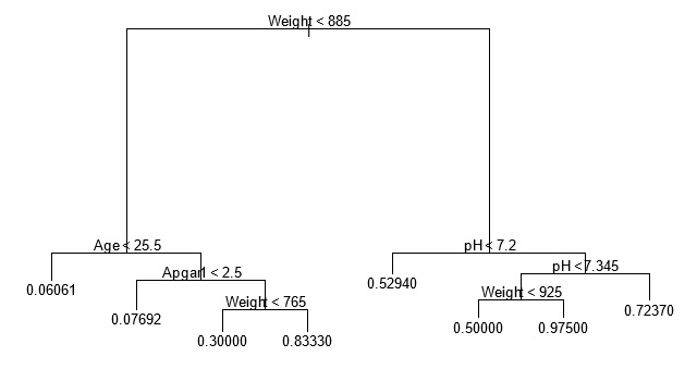
If we choose GLMs, we would try various links and go through variable selection procedures (and perform diagnostics along the way, such as Areas under ROC curves or confusion tables). One key issue, though, is whether there are interactions between the gestational age variable and the others, since if there are that would mean the survival rate change for a change in gestational age from 30 to 31 weeks would depend on the actual values of the other predictors, and we are only told to assume they wouldn’t change, but not their actual values. We might just check a bunch of interactions manually by directly including them in our GLM, or instead fit a tree model and see what, if any, interactions it can pick up automatically. Now, if we fit a tree model, use cross-validation and prune it back, we get the following:

> bby <- read.table("bby.day",header=T)

> library(tree)

> bby.tree <- tree(Survival ~ .,data=bby)

> order(cv.tree(bby.tree)$dev)

[1] 8

> plot(prune.tree(bby.tree,best=8)

So, it appears there is some potential interactions, since pH is only an important factor for larger birthweight babies, while age and Apgar1 are the important factors for low birthweight babies. Fortunately, (via deviance testing or other model selection techniques), only the pH/Weight interaction appears significant. So, the quantity in question is determined just by the coefficient of the gestational age predictor. How we turn this into a confidence interval for the change in survival chances depends on our link structure. As an example, suppose we fit a logistic link model and the coefficient in question is 𝛽̂_𝑎𝑔𝑒 with standard deviation of 𝑠𝑒(𝛽̂_𝑎𝑔𝑒). Then, 𝛽̂_𝑎𝑔𝑒 represents the change in the log-odds of survival for a 1 week change in gestational age:

ln{𝜋̂₃₁/(1 − 𝜋̂₃₁)} − ln{𝜋̂₃₀/(1 − 𝜋̂₃₀)} = 𝛽̂_𝑎𝑔𝑒

which rearranges to:

𝜋̂31(1 − 𝜋̂30) 𝛽̂𝑎𝑔𝑒

-------------------------------= 𝑒

𝜋̂₃₀(1 − 𝜋̂₃₁)

So, a confidence interval for the odds would be 𝑒^𝛽̂^𝑎𝑔𝑒^{±1.96𝑠𝑒(𝛽̂}^𝑎𝑔𝑒⁾. Alternatively, for a CI for some other form, we could use the delta method to determine an appropriate standard deviation.

b) Apgar scores are valued on an 11-point scale. Initially, we might think of using continuous response models (and fitting them would certainly have gotten some marks, if done properly), but a better approach here is to use a model for ordinal responses.

> library(MASS)

> bby$Apgar5 <- factor(bby$Apgar5,

+ levels=c("0","1","2","3","4","5","6","7","8","9","10"),

+ ordered=T)

> bby.pol1 <- polr(Apgar5 ~ .,method="logistic",data=bby)

> summary(bby.pol1)

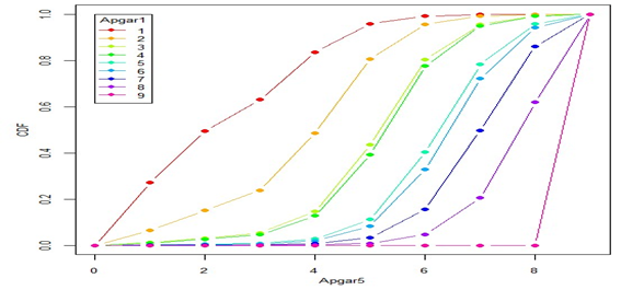
Fitting a proportional odds logistic regression for the distribution of five minute Apgar score shows that Age and Weight are not significant once we have included the 1 minute Apgar score in the model. Further, there are clearly some issues with categories 0 and 10. A quick table shows that there are only 4 values of 0 and a single value of 10 in the entire dataset. So, we should probably combine these end categories with the one next to them, as the analysis will be unstable if it has to fit categories with such low numbers of observations. If we re-fit the model without Age and Weight and with the updated Apgar score variables, we can see the fitted CDFs of Apgar5 for each value of Apgar1:

> A5 <- ifelse(bby$Apgar5==0,1,ifelse(bby$Apgar5==10,9,bby$Apgar5))

> A1 <- ifelse(bby$Apgar1==0,1,bby$Apgar1)

> apgar.tbl <- as.vector(table(A5,A1))

> a5 <- factor(rep(1:9,9),levels=1:9,ordered=T)

> a1 <- factor(as.character(rep(1:9,rep(9,9))))

> bby.pol2 <- polr(a5 ~ a1,weights=apgar.tbl)

> fitp <- bby.pol2$fitted.values[seq(1,81,9),]

> fitF <- apply(cbind(0,fitp),1,cumsum)

> matplot(0:9,fitF,type="b",lty=1,pch=16,col=rainbow(9),xlab="Apgar5",

+ ylab="CDF")

> legend(0,1,legend=as.character(1:9),title="Apgar1",lty=1,pch=16,

+ col=rainbow(9))

Alternatively, we could ignore the ordinal nature and consider Apgar scores as just categorical and then we could use classification or discrimination techniques to predict Apgar scores. (NOTE: It is even tempting to consider Apgar scores as continuous given they have so many categories, but this is not appropriate.)

Question 3:(18 Total Marks)

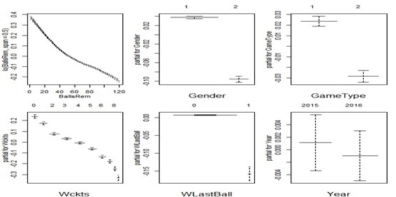
a) Runs per over is a count variable, so Poisson regression is a reasonable way to go here (although continuous response models would also work as long as we were careful about the fact that we cannot have negative values for our response variable, so an appropriate link structure such as the natural logarithm would be needed); however, we are ultimately asked for some graphical depictions of our relationship, so some spline or local regression methods will also be useful. To do both, we can use a GAM model. (NOTE: A bit of investigation shows the runs distribution is skewed, but also has lots of zeroes, so we can’t use a log-link, and thus a square-root link seems the best approach).

> ckt <- read.table("crkt.dat",header=T,sep=" ")

> ckt120 <- ckt[ckt$BallsRem<=120,]

> ckt120$Gender <- as.factor(ckt120$Gender)

> ckt120$GameType <- as.factor(ckt120$GameType)

> ckt120$Year <- as.factor(ckt120$Year)

> ckt120$WLastBall <- as.factor(ckt120$WLastBall)

> ckt120$Wckts <- as.factor(ckt120$Wckts)

> par(mfrow=c(2,3))

> ckt120.gam <- gam(Runs ~ lo(BallsRem,span=0.5) + Gender + GameType +

+ + Wckts + WLastBall + Year,

+ family=poisson(link=sqrt),data=ckt120)) > plot(ckt120.gam)

So, it does appear that there is a significant difference between the two game types. However, the practical implications of this statistical result (which is significant in part due to the huge sample size) seems very small (it is on the order of 0.05 of a run!).

b) We could just use the above analysis, and it again shows that a wicket on the last ball creates a statistically significant drop in average runs scored on the next ball, but the size of the drop is again not that practically important (on the order of 0.15 runs per ball). Alternatively, we could use a Poisson GLM to investigate whether there are any interactions.

Resources

24 x 7 Availability.
Trained and Certified Experts.
Deadline Guaranteed.
Plagiarism Free.
Privacy Guaranteed.
Free download.
Online help for all project.
Homework Help Services

Not the Exact Question you were looking for ? Post your question for assignment help and get instant help on your homework and assignment questions from our experts