STAT20029 Module 6 Continuous distributions
Module 6: Continuous distributions
Introduction
This week we will look at three distributions where the random variable can take on any value on a continuum. These are called continuous distributions. This allows the exploration of the distribution of objects or processes that involve continuous measurements, (such as height, weight, time, distance). Examples are the number of kilometres a car can travel per litre of petrol, the amount of money a corporation invests in charity events, the number of megabytes of hard-disk space employees of a company use to store computer files, the weight of a shipment etc. The weight can be 1.2 tons, 1.213 tons or 1.21354397... tons depending on the accuracy one desires.
The first distribution we will examine this week is the normal distribution. This is often referred to as the ‘bell-shaped curve’ and describes a surprising number of variables quite well. Often it is used to model the distribution of student’s grades in an exam (hence the American expression ‘grading on the curve’), the heights of men or the heights of women (which follow separate normal distributions) and fill weights of grocery packaging (for example, cereal boxes), etc.
The second distribution is the uniform distribution. As its name suggests, this distribution takes on uniform values across its domain. In other words, every outcome is equally likely.
The final distribution we will look at this week is the exponential distribution. This is often used to describe such things as arrival times (for example, the arrival of people at an ATM).
Objectives
On completion of this module you should be able to:
- calculate areas under the standard normal curve
- solve and interpret problems involving the normal distribution
- check assumptions of normality
- calculate probabilities using the uniform distribution,
- solve and interpret problems involving the uniform distribution
- calculate probabilities using the exponential distribution and
- solve and interpret problems involving the exponential distribution.
Continuous random variables
Random variables that can take on any value on a continuum are called continuous random variables. The height of people, for example, is regarded as a continuous random variable. Although measuring equipment (such as a tape measure in this case) only gives a certain degree of accuracy, the more accurate the measuring equipment, the more accurate the measure of a person’s height will be. Other examples include the current outdoor temperature, income, IQ (intelligence quotient) score, monthly amount a company spends on advertising, etc.
With discrete random variables, it made sense to associate a certain probability with each possible outcome of the random variable. This was called a discrete probability distribution. With continuous random variables, however, since there are an infinite number of possible values that the random variable might take on, it makes no sense to attempt to associate a probability with each one! Instead, probabilities are associated with intervals on the continuum.
For example, imagine staff at a particular company are required to complete a short online survey about working conditions. The time taken for each staff member to complete the survey is recorded in seconds (including a number of decimal places based on parts of seconds). The graph below displays the probability density function of the times to complete the questionnaire. From this graph we can see that most employees took between about 60 and 180 seconds to complete the questionnaire. The probability that an employee takes between 140 and 160 seconds is shaded on the graph. This corresponds to a probability of 0.1359.
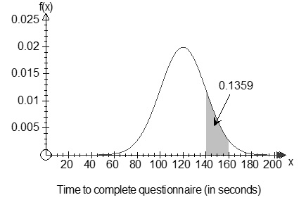
Given sufficient information about the distribution itself (i.e., the mathematical formula), we could also calculate the probabilities for any other intervals. The graph is actually a normal distribution with a mean of 120 seconds and a standard deviation of 20 seconds. As an exercise, when you have covered the material on the normal distribution that follows, return to this example and verify the probability displayed on the graph.
A mathematical function for the curve pictured above is called a probability density function. A probability density function for a continuous random variable, X, is a mathematical function for which the area under the curve corresponding to any interval is equal to the probability that X will take on a value in the interval. The probability density function is denoted by f(x), which indicates the probability density at x.
This week we will examine three key continuous probability density functions: the uniform distribution, the normal distribution and the exponential distribution.
Graphs of these distributions follow:

The uniform distribution
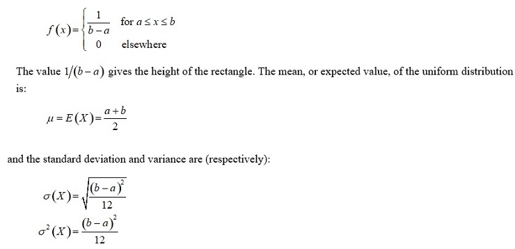
The uniform distribution, or rectangular distribution, is so called because of its rectangular shape. It is described by two parameters, a and b, where a is the smallest value that X can assume and b is the largest value that X can assume. The continuous uniform probability density function is:
Example 6–1
A surfer knows that the time between wipe-outs (falling off his surfboard) is uniformly distributed between two minutes and nine minutes in particularly large surf. What is the probability that the time between wipe-outs is:
(a) less than five minutes
(b) between three and four minutes
(c) more than six minutes
(d) What is the expected value of the time between wipe-outs?
(e) What is the standard deviation of the time between wipe-outs?
The normal distribution
The normal distribution is one of the most important distributions in classical statistics, having applications in a variety of fields. In the introduction, we mentioned the following examples of variables that can be described by a normal distribution: student’s grades in an exam, the heights of men or the heights of women and fill weights of grocery packaging. Note that “normal distribution” is just a name – it has nothing to do with being normal or abnormal.
The normal distribution is described by two parameters: the mean (μ) and standard deviation (α). The normal random variable may take on any value between -∞ and +∞. Although most real-world examples have limits on the value the variable can take, the normal model is often still useful in these situations.
The normal probability density function is denoted by:
f(x)=1/(√2πσ) exp[-1/2 ((x-μ)/σ)2]
where π=3.14159... and the exp notation means exp[a]=ea where e=2.71828... is the base of natural logarithms. The normal distribution’s distinctive bell shape has its centre (and peak) at the mean, μ. The parameter α, the standard deviation, determines the spread of the distribution. Since the equation given above is quite complex, you will never have to use this equation, instead you will always be using the standard normal table for solving problems related to normal distribution. Because a normal distribution is uniquely defined by its mean and standard deviation (or variance), the following notation is often used to denote a particular normal distribution: N(μ,σ2 ). Some examples of the normal distribution curves are given below.
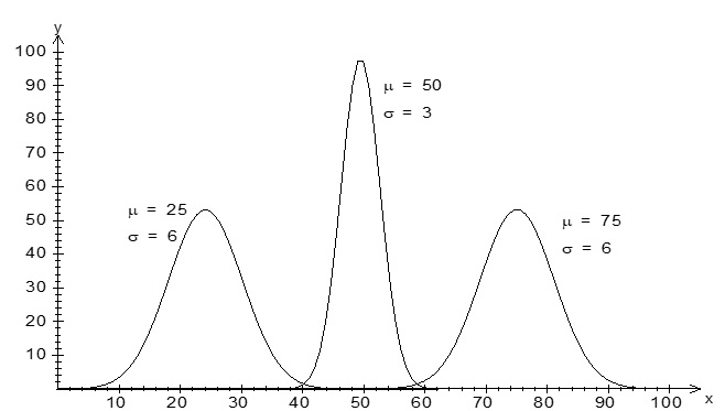
The standard normal distribution is a particular example of the normal distribution with μ=0 and σ=1. The standard normal random variable is denoted by Z. Using the notation mentioned above, we can say that Z is distributed as N(0,1). The standardised form of a normal random variable X with mean μ and standard deviation α is:
Z=(X-μ)/σ
This formula is useful to us, since standard normal probabilities tables can be used to find probabilities (see Table A.5 in the text). It means we are not forced to evaluate the (rather messy) normal probability density function each time we want to calculate a probability. We use a lower case z to indicate a particular outcome of the standard normal random variable Z. The tables in the text used in this course giveP(0< Z< z). Since the standard normal curve is symmetric, only the values for the right half of the curve is given. Table A.6 on page 769 provide the cumulative values.
Example 6–2
Evaluate the following probabilities for the standard normal variable, Z:
- P(Z≤1)
- P(Z≤-2.76)
- P(Z≥1.49)
Determining probabilities for any normal distribution
The standard normal distribution tables can be used to calculate probabilities for any normal random variable. This is done by transforming the normal random variable, X, into the standard normal variable, Z using the linear transformation Z=(X-μ)/σ. We’ll demonstrate with an example.
Example 6–3
A final exam for a particular accountancy course is known by students to be a difficult one. In the past, the mean mark was 62% and the standard deviation was 11%. What proportion of students have received a mark of:
- at least 65%
- at least 50%
- less than 40%
- between 70% and 100%
Between what two marks symmetrically distributed around the mean will 95% of the students’ marks fall?
Checking the assumption of normality
In order to be able to use the normal distribution in real-world examples, we must first test to see whether data can be approximated by the normal distribution. We do this by checking to see whether the characteristics of the data set match those of a normal distribution and by producing a normal probability plot.
The normal distribution has the following characteristics:
- it is symmetrical
- it is bell-shaped
- the mean, median and mode are equal
- the interquartile range equals 1.33 standard deviations.
We can test visually for symmetry and a bell-shape using a histogram (or stem-and-leaf plot for smaller data sets) and using a box-and-whisker plot. We obviously need to use numerical summaries to test for equality of mean, median and mode and to compare the interquartile range to 1.33 standard deviations. We shall demonstrate these in Example 6–4 below.
For a more thorough investigation, we might also examine other characteristics of a normal distribution. For example, we can show that
- approximately 68.26% of the values of a normal distribution fall within ±1 standard deviation of the mean
- approximately 95.44% of the values of a normal distribution fall within ±2 standard deviation of the mean
- approximately 99.73% of the values of a normal distribution fall within ±3 standard deviation of the mean.
The normal probability plot is another useful tool in determining the appropriateness of the normal distribution. In practice, normal probability plots are most often produced by a computer because they tend to be quite messy to produce by hand. However, we will explain how the graph is produced, since it is essential to understand what the software is doing!
Creating a normal probability plot:
- Rank the data from smallest to largest value, giving the smallest observation rank 1 through to the largest with rank n.
- For each rank, i=1,…,n, find the percentile of order i/((n+1) ). For example, if the sample size is , these values will be 1/((50+1) )=0.0196, 2/((50+1) )=0.0392, …, 50/((50+1) )=0.9804 (all to 4 decimal places).
- Find the standard normal distribution values, Zi which correspond to the cumulative area of these values. For example, Z0.0196=-2.06 (found by looking for 0.0196 in the body of the standard normal table), Z0.0392=-1.76 through to Z0.9804=2.06.
- Produce a scatterplot of the ordered data values against the standardised normal scores.
If the data are normally distributed, the normal probability plot should fall along a straight line, with the slope of the line given by 1/σ. The graphs below indicate the approximate shapes we might expect for normally distributed data, left-skewed data, right-skewed data and rectangular-shaped distribution data.
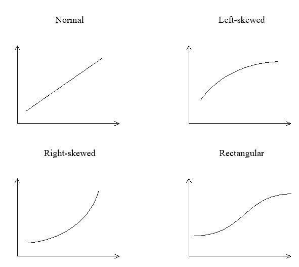
Normal probability plot is a reliable technique for testing for normality. If this procedure is followed there is no need to do other tests mentioned earlier such as boxplot, interquartile range, etc.
|
Example 6–4 Last term, a group of 21 students enrolled in an accounting course on a particular campus. Their scores on the final exam are recorded below. Determine whether or not these marks are normally distributed by evaluating the actual versus theoretical properties and by constructing a normal probability plot.
|
The exponential distribution
The exponential distribution has a distinct right-skewed shape which is useful in describing duration phenomena. For example, the random variable X might represent the time until a caller waiting in a queue has their call answered or the time until the arrival of the next customer at a particular ATM. The exponential random variable may take on any positive value: 0< x <∞.. The exponential distribution has one parameter, λ, which represents the mean number of arrivals per unit. This parameter is always positive: λ>0. The exponential cumulative probability density function is:
P(X < x) = 1-e-2x
As an example, imagine we know that on average three customers call a customer helpline each minute. Therefore we have λ=3. Then, if we wished to find the probability that the next call occurred within 15 seconds (i.e., 0.25 minutes), we would be looking for P(X<0.25)=1-e^(-3(0.25) )="0.5276" (to 4 decimal places). Exponential distribution belongs to the Poisson process. If we are looking for a discrete variable such as number of people arriving at an ATM in a given time interval, we use the Poisson distribution. However, if we are dealing with a continuous variable such as time between arrival, we use exponential distribution.
The mean of an exponential distribution is 1/λ and the standard deviation is also 1/λ.
Example 6–5
People are known to arrive at a particular vending machine at a mean rate of 27 per hour. Assuming that these arrival times follow an exponential distribution, find the probability that the next person will arrive:
- within one minute
- within five minutes
- in more than five minutes
Note probability is a dimensionless number. Therefore, if x is in minutes, λ must be in per minute so that minute dimensions cancel each other.
Discussion points
|
Discussion point 6–1 In this unit, you will never use the formula for the density function of the normal distribution because mathematically it is challenging to find the area under the curve. Instead, you have to use the standard normal table. Discuss how to find areas under the normal curve using the table. Discussion point 6–2 A friend comes to you and makes the statement that ‘anything we measure in the real world is effectively continuous and can be modelled by a normal distribution’. How would you respond? With other students, discuss, compare and justify your answer. |
Summary
Now that you have completed this module, turn back to the objectives at the beginning of the module. Have you achieved these objectives?
Ensure that you attempt the recommended problems in the list of review questions below and at least a sample of problems from the optional list. This will help you to identify any areas of difficulty you have in achieving the module’s objectives.
Review questions
Recommended problems
Black et al. : Do Questions 6.6 on page 201, 6.7 and 6.12 on page 202, 6.13 on page 205, 6.16 on page 209, 6.22 and 6.25 on page 211, 6.2 on page 213, 6.8 on page 214.
Optional problems
Black et al. : Choose a selection of problems from Questions 6.3 on page 198, 6.11 on page 202, 6.15 on page 208, 6.17 on page 209, 6.21 and 6.23 on page 211, 6.4 on page 213, 6.9 on page 214.
Tutorial and Workshop
Workshop
A Practical Example
Problem demonstrating probability estimations for a continuous variable:
The triangle in Figure 6.1 represents the probability distribution of a continuous random variable.
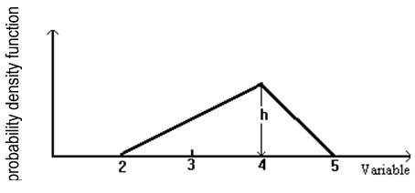
Figure 6.1 Triangular probability distribution.
(a) What should be the value of height “h” for the triangle to represent a probability distribution?
(b) What is the probability of the random variable falling between 3 and 4?
Tutorial
Solve the recommended problems under Review questions.

