The application of a one-way analysis of variance
11 ANALYSIS OF VARIANCE
CHAPTER LEARNING OBJECTIVES
- Explain the application of a one-way analysis of variance (ANOVA) model.
- Define the concepts of between and within total variance.
- Calculate and interpret a test for two or more sample cases with means.
- Determine the significance of an F-ratio test statistic.
- Interpret output for ANOVA.
Many research questions require us to look at multiple samples or groups, at least more than two at a time. We may be interested in studying the relationship between ethnic identity (white, African American, Asian American, Latino) and church attendance, the influence of one’s social class (lower, working, middle, and upper) on President Donald Trump’s job approval ratings, or the effect of educational attainment (less than high school, high school graduate, some college, and college graduate) on household income. Note that each of these examples requires a comparison between multiple demographic or ethnic groups, more than the two-group comparisons we reviewed in Chapter 8. While it would be easy to confine our analyses between two groups, our social world is much more complex and diverse.
Let’s say that we’re interested in examining educational attainment—on average, how many years of education do Americans achieve? For 2018, the U.S. Census reported that 89.8% of adults (25 years and older) completed at least a high school degree, and 35% of all adults attained at least a bachelor’s degree.1 Special attention has been paid to the educational achievement of Latino students. Data from the U.S. Census, as well as from the U.S. Department of Education, confirm that Latino students continue to have lower levels of educational achievement than other racial or ethnic groups.
In Chapter 8, we introduced statistical techniques to assess the difference between two sample means or proportions. In Table 8.2, we compared the difference in educational attainment for blacks and whites. But what if we wanted to examine more than two racial or ethnic groups?
Suppose we collect a random sample of 23 men and women, grouped them into four demographic categories, and included their educational attainment in Table 11.1. With the t-test statistic we discussed in Chapter 8, we could analyze only two samples at a time. We would have to analyze the mean educational attainment of whites and blacks, whites and Asians, whites and Latinos, blacks and Asians, and so on. (Confirm that we would have to analyze six different pairs.) In the end, we would have a series of t-test statistic calculations, and we still wouldn’t be able to answer our original question: Is there a difference in educational attainment among all four demographic groups?
Table 11.1 Educational Attainment (Measured in Years) for Four Racial/Ethnic Groups
|
White |
Black |
Asian |
Latino |
|
n1 = 6 |
n2 = 5 |
n3 = 6 |
n4 = 6 |
|
12 |
16 |
16 |
11 |
|
12 |
12 |
18 |
12 |
|
14 |
13 |
16 |
12 |
|
12 |
13 |
14 |
13 |
|
12 |
14 |
16 |
16 |
|
16 |
20 |
11 |
Source: U.S. Census Bureau, Educational Attainment in the United States: 2018, Table 1.
LEARNING CHECK 11.1
Identify the independent and dependent variables in Table 11.1.
There is a statistical technique that will allow us to examine all the four groups or samples simultaneously. This technique is called analysis of variance (ANOVA). ANOVA follows the same five-step model of hypothesis testing that we used with t test for means and Z test for proportions (in Chapter 8) and chi-square (in Chapter 10). In this chapter, we review the calculations for ANOVA and discuss two applications of ANOVA from the research literature.
Analysis of variance (ANOVA): An inferential statistics technique designed to test for the significant relationship between two variables in two or more groups or samples.
UNDERSTANDING ANALYSIS OF VARIANCE
Recall that the t test examines the difference between two means, ¯¯¯Y1−¯¯¯Y2Y¯1−Y¯2 , while the null hypothesis assumed that there was no difference between them: μ1 = μ2. Rejecting the null hypothesis meant that there was a significant difference between the two mean scores (or the populations from which the samples were drawn).
The logic of ANOVA is the same but extending to two or more groups. For the data presented in Table 11.1, ANOVA will allow us to examine the variation among four means (¯¯¯Y1,¯¯¯Y2,¯¯¯Y3,¯¯¯Y4)(Y¯1,Y¯2,Y¯3,Y¯4) , and the null hypothesis can be stated as follows: μ1 = μ2 = μ3 = μ4. Rejecting the null hypothesis for ANOVA indicates that there is a significant variation among the four samples (or the four populations from which the samples were drawn) and that at least one of the sample means is significantly different from the others. In our example, it suggests that years of education (dependent variable) do vary by group membership (independent variable).
When ANOVA procedures are applied to data with one dependent and one independent variable, it is called a one-way ANOVA.
One-way ANOVA: Analysis of variance application with one dependent variable and one independent variable.
The means, standard deviations, and variances for the samples have been calculated and are shown in Table 11.2. Note that the four mean educational years are not identical, with Asians having the highest educational attainment. Also, based on the standard deviations, we can tell that the samples are relatively homogeneous with deviations within 1.51 to 2.07 years of the mean. We already know that there is a difference between the samples, but the question remains: Is this difference significant? Do the samples reflect a relationship between demographic group membership and educational attainment in the general population?
LEARNING CHECK 11.2
We’ve calculated the mean and standard deviation scores for each group in Table 11.2. Compute each mean (Chapter 3) and standard deviation (Chapter 4) and confirm that our statistics are correct.
To determine whether the differences are significant, ANOVA examines the differences between our four samples, as well as the differences within a single sample. The differences can also be referred to as variance or variation, which is why ANOVA is the analysis of variance. What is the difference between one sample’s mean score and the overall mean? What is the variation of individual scores within one sample? Are all the scores alike (no variation), or is there a broad variation in scores? ANOVA allows us to determine whether the variance between samples is larger than the variance within the samples. If the variance is larger between samples than the variance within samples, we know that educational attainment varies significantly across the samples. It would support the notion that group membership explains the variation in educational attainment.
Table 11.2 Years of Education, Means, Standard Deviations, and Variances for Four Racial/Ethnic Groups
|
White |
Black |
Asian |
Latino |
|
n1 = 6 |
n2 = 5 |
n3 = 6 |
n4 = 6 |
|
12 |
16 |
16 |
11 |
|
12 |
12 |
18 |
12 |
|
14 |
13 |
16 |
12 |
|
12 |
13 |
14 |
13 |
|
12 |
14 |
16 |
16 |
|
16 |
— |
20 |
11 |
|
¯¯¯Y1=13.00Y¯1=13.00 |
¯¯¯Y2=13.60Y¯2=13.60 |
¯¯¯Y3=16.67Y¯3=16.67 |
¯¯¯Y4=12.50Y¯4=12.50 |
|
s1 = 1.67 |
s2 = 1.51 |
s3 = 2.07 |
s4 = 1.87 |
|
s21=2.79s12=2.79 |
s22=2.28s22=2.28 |
s23=4.28s32=4.28 |
s24=3.50s42=3.50 |
|
¯¯¯Y(forallgroups)=13.96Y¯(forallgroups)=13.96 |
THE STRUCTURE OF HYPOTHESIS TESTING WITH ANOVA
The Assumptions
ANOVA requires several assumptions regarding the method of sampling, the level of measurement, the shape of the population distribution, and the homogeneity of variance.
Independent random samples are used. Our choice of sample members from one population has no effect on the choice of sample members from the second, third, or fourth population. For example, the selection of Asians has no effect on the selection of any other sample.
The dependent variable, years of education, is an interval-ratio level of measurement. Some researchers also apply ANOVA to ordinal-level measurements.
The population is normally distributed. Although we cannot confirm whether the populations are normal, given that our N is so small, we must assume that the population is normally distributed to proceed with our analysis.
The population variances are equal. Based on our calculations in Table 11.2, we see that the sample variances, although not identical, are relatively homogeneous.2
Stating the Research and the Null Hypotheses and Setting Alpha
The research hypothesis (H1) proposes that at least one of the means is different. We do not identify which one(s) will be different, or larger or smaller; we only predict that a difference does exist.
H1: At least one mean is different from the others.
ANOVA is a test of the null hypothesis of no difference between any of the means. Since we’re working with four samples, we include four μs in our null hypothesis.
H0: μ1 = μ2 = μ3 = μ4
As we did in other models of hypothesis testing, we’ll have to set our alpha. Alpha is the level of probability at which we’ll reject our null hypothesis. For this example, we’ll set alpha at .05.
The Concepts of Between and Within Total Variance
A word of caution before we proceed: Since we’re working with four different samples and a total of 23 respondents, we’ll have a lot of calculations. It’s important to be consistent with your notations (don’t mix up numbers for the different samples) and be careful with your calculations.
Our primary set of calculations has to do with the two types of variance: (1) between-group variance and (2) within-group variance. The estimate of each variance has two parts, the sum of squares and degrees of freedom (df).
The between-group sum of squares (SSB) measures the difference in average years of education between our four groups. Sum of squares is the abbreviation for “sum of squared deviations.” For SSB, what we’re measuring is the sum of squared deviations between each sample mean to the overall mean score. The formula for the SSB can be presented as follows:
Between-group sum of squares (SSB): The sum of squared deviations between each sample mean to the overall mean score.
(11.1)
SSB=∑nk(¯¯¯Yk−¯¯¯Y)2SSB=∑nk(Y¯k−Y¯)2
where
- nk = the number of cases in a sample (k represents the number of different samples)
- ¯¯¯YkY¯k = the mean of a sample
- ¯¯¯YY¯ = the overall mean
SSB can also be understood as the amount of variation in the dependent variable (years of education) that can be attributed to or explained by the independent variable (the four demographic groups).
Within-group sum of squares (SSW) measures the variation of scores within a single sample or, as in our example, the variation in years of education within one group. SSW is also referred to as the amount of unexplained variance, since this is what remains after we consider the effect of the specified independent variable. The formula for SSW measures the sum of squared deviations within each group, between each individual score with its sample mean.
Within-group sum of squares (SSW): Sum of squared deviations within each group, calculated between each individual score and the sample mean.
(11.2)
SSW=∑(Yi−¯¯¯Yk)2SSW=∑(Yi−Y¯k)2
where
- Yi = each individual score in a sample
- ¯¯¯YkY¯k = the mean of a sample
Even with our small sample size, if we were to use Formula 11.2, we’d have a tedious and cumbersome set of calculations. Instead, we suggest using the following computational formula for within-group variation or SSW:
(11.3)
SSW=∑Y2i−∑(∑Yk)2nkSSW=∑Yi2−∑(∑Yk)2nk
where
- Y2iYi2 = the squared scores from each sample
- ΣYkΣYk = the sum of the scores of each sample
- nk = the number of cases in a sample
Together, the explained (SSB) and unexplained (SSW) variances compose the amount of total variation in scores. The total sum of squares (SST) can be represented by
Total sum of squares (SST): The total variation in scores, calculated by adding SSB (between-group sum of squares) and SSW (within-group sum of squares).
(11.4)
SST=∑(Yi−¯¯¯Y)2=SSB+SSWSST=∑(Yi−Y¯)2=SSB+SSW
where
- Yi = each individual score
- ¯¯¯YY¯ = the overall mean
The second part of estimating the between-group and within-group variances is calculating the degrees of freedom. Degrees of freedom are also discussed in Chapters 8 and 10. For ANOVA, we have to calculate two degrees of freedom. For SSB, the degrees of freedom are determined by
dfb = k – 1 (11.5)
where k is the number of samples.
For SSW, the degrees of freedom are determined by
dfw = N – k (11.6)
where
- N = total number of cases
- k = number of samples
Finally, we can estimate the between-group variance by calculating mean square between. Simply stated, mean squares are averages computed by dividing each sum of squares by its corresponding degrees of freedom. Mean square between can be represented by
Mean square between: Sum of squares between divided by its corresponding degrees of freedom.
Mean square between = SSB / dfb (11.7)
and the within-group variance or mean square within can be represented by
Mean square within: Sum of squares within divided by its corresponding degrees of freedom.
Mean square within = SSW / dfw (11.8)
The F Statistic
Together, the mean square between (Formula 11.7) and mean square within (Formula 11.8) compose the F ratio obtained or F statistic. Developed by R. A. Fisher, the F statistic is the ratio of between-group variance to within-group variance and is determined by Formula 11.9:
F ratio or F statistic: The test statistic for ANOVA, calculated by the ratio of mean square to mean square within.
(11.9)
F=MeansquarebetweenMeansquarewithin=SSB/dfbSSW/dfwF=MeansquarebetweenMeansquarewithin=SSB/dfbSSW/dfw
We know that a larger F-obtained statistic means that there is more between-group variance than within-group variance, increasing the chances of rejecting our null hypothesis. In Table 11.3, we present additional calculations to compute F.
Table 11.3 Computational Worksheet for ANOVA
|
White |
Black |
Asian |
Latino |
|
n1 = 6 |
n2 = 5 |
n3 = 6 |
n4 = 6 |
|
12 |
16 |
16 |
11 |
|
12 |
12 |
18 |
12 |
|
14 |
13 |
16 |
12 |
|
12 |
13 |
14 |
13 |
|
12 |
14 |
16 |
16 |
|
16 |
— |
20 |
11 |
|
¯¯¯Y1=13.00Y¯1=13.00 |
¯¯¯Y2=13.60Y¯2=13.60 |
¯¯¯Y3=16.67Y¯3=16.67 |
¯¯¯Y4=12.50Y¯4=12.50 |
|
s1 = 1.67 |
s2 = 1.51 |
s3 = 2.07 |
s4 = 1.87 |
|
S21=2.79S12=2.79 |
s22=2.28s22=2.28 |
s23=4.28s32=4.28 |
s24=3.50s42=3.50 |
|
Y1 = 78 |
Y2 = 68 |
Y3 = 100 |
Y4 = 75 |
|
Y21=1028Y12=1028 |
Y22=934Y22=934 |
Y23=1,688Y32=1,688 |
Y24=955Y42=955 |
|
¯¯¯Y(forallgroups)=13.96Y¯(forallgroups)=13.96 |
Let’s calculate between-group sum of squares and degrees of freedom based on Formulas 11.1 and 11.5. The calculation for SSB is
∑nk(Y−Y)2=6(13−13.96)2+5(13.6−13.96)2+6(16.67−13.96)2+6(12.5−13.96)2∑nk(Y−Y)2=6(13−13.96)2+5(13.6−13.96)2+6(16.67−13.96)2+6(12.5−13.96)2
= 5.53 + .65 + 44.06 + 12.79
= 63.03
The degrees of freedom for SSB is k – 1 or 4 – 1 = 3. Based on Formula 11.7, the mean square between is
Mean square between = 63.03 / 3 = 21.01
The within-group sum of squares and degrees of freedom are based on Formulas 11.3 and 11.6. The calculation for SSW is
∑Y2i−∑(ΣYk)2nk=(1,028+934+1,688+955)−(7826+6825+10026+7526)∑Yi2−∑(ΣYk)2nk=(1,028+934+1,688+955)−(7826+6825+10026+7526)
= 4,605 – (1,014 + 924.8 + 1,666.67 + 937.50)
= 4,605 – 4,542.97
= 62.03
The degrees of freedom for SSW is N – k = 23 – 4 = 19. Based on Formula 11.8, the mean square within is
Mean square within = 62.03 / 19 = 3.26
Finally, our calculation of F is based on Formula 11.9:
F ratio = 21.01 / 3.26 = 6.44
A Closer Look 11.1Decomposition of SST
According to Formula 11.4, sum of squares total (SST) is equal to
SST=∑(Yi−¯¯¯Y)2=SSB+SSWSST=∑(Yi−Y¯)2=SSB+SSW
You can see that the between sum of squares (explained variance) and within sum of squares (unexplained variance) account for the total variance (SST) in a particular dependent variable. How does that apply to a single case in our educational attainment example? Let’s take the first black respondent in Table 11.1 with 16 years of education.
This respondent’s total deviation (corresponding to SST) is based on the difference between the years of education from the overall mean (Formula 11.4). The individual mean is quite a bit higher than the overall mean education of 8 years. The difference of the individual from the overall mean is 2.04 years (16 – 13.96). Between-group deviation (corresponding to SSB) can be determined by measuring the difference between the group average from the overall mean (Formula 11.1). The deviation between the group average and overall average for blacks is –.36 years (13.60 – 13.96). Finally, the within-group deviation (corresponding to SSW, Formula 11.2) is based on the difference between the first black person’s years of education and the group average for blacks: 2.40 years (16 – 13.60). So for the first black person in our sample, SSB + SSW = SST or 2.40 + –.36 = 2.04. In a complete ANOVA problem, we’re computing these two sources of deviation (SSB and SSW) to obtain SST (Formula 11.4) for everyone in the sample.
Making a Decision
To determine the probability of calculating an F statistic of 6.44, we rely on Appendix E, the distribution of the F statistic. Appendix E lists the corresponding values of the F distribution for various degrees of freedom and two levels of significance, .05 and .01.
Since we set alpha at .05, we’ll refer to the table marked “p = .05.” Note that Appendix E includes two dfs. These refer to our degrees of freedom, df1 = dfb and df2 = dfw.
Because of the two degrees of freedom, we’ll have to determine the probability of our F obtained differently than we did with t test or chi-square. For this ANOVA example, we’ll have to determine the corresponding F, also called the F critical, when dfb = 3 and dfw = 19, and α = .05.
Based on Appendix E, the F critical (as in Appendix E) is 3.13, while our F obtained (the one that we calculated) is 6.44. Since our F obtained is greater than the F critical (6.44 > 3.13), we know that its probability is <.05, extending into the shaded area. (If our F obtained was <3.13, we could determine that its probability was greater than our alpha of .05, in the unshaded area of the F-distribution curve. Refer to Figure 11.1.) We can reject the null hypothesis of no difference and conclude that there is a significant difference in educational attainment between the four groups.
F critical: F-test statistic that corresponds to the alpha level, dfw, and dfb.
F obtained: The F-test statistic that is calculated.
THE FIVE STEPS IN HYPOTHESIS TESTING: A SUMMARY
To summarize, we’ve calculated an ANOVA test examining the difference between four demographic groups and their average years of education.
- Making Assumptions:
- Independent random samples are used.
- The dependent variable, years of education, is an interval-ratio level of measurement.
- The population is normally distributed.
- The population variances are equal.
- Stating the Research and Null Hypothesis and Selecting Alpha:
- H1: At least one mean is different from the others.
H0: μ1 = μ2 = μ3 = μ4
α = .05
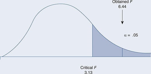
Figure 11.1 Comparing F Obtained Versus F Critical
Selecting the Sampling Distribution and Specifying the Test Statistic: The F distribution and F statistic are used to test the significance of the difference between the four sample means.- Computing the Test Statistic: We need to calculate the between-group and within-group variation (sum of squares and degrees of freedom). We estimate SSB = 21.01 (dfb = 3) and SSW = 3.26 (dfw = 19).
Based on Formula 11.9,
F = 21.01 / 3.26 = 6.44
- Making a Decision and Interpreting the Results: We reject the null hypothesis of no difference. Our F obtained of 6.44 is greater than the F critical of 3.13. The probability of 6.44 is <.05. F doesn’t advise us about which groups are different, only that educational attainment does differ significantly by demographic group members. Based on the sample data, we know that the only group to achieve a college education average was Asians (16.67 years). If we were to rank the other group means, second highest educational attainment was among blacks (13.60), followed by whites (13.00) and Latinos (12.50).
LEARNING CHECK 11.3
If alpha were changed to .01, would our final decision change?
STATISTICS IN PRACTICE: THE ETHICAL CONSUMER
Consumers increasingly avoid products that are perceived as having a negative social or environmental impact. By purchasing fair labor, organic, or environmentally safe products, consumers express their politics through their purchases, a practice that has been referred to as ethical consumerism. The GSS 2014 included a series of questions on what it takes to be a good citizen. Respondents were asked how important it was to “choose products for political, ethical or environmental reasons, even if they cost a bit more.” Answers were ranked on a 7-point scale: 1 = not at all important to 7 = very important. We use SPSS and the GSS 2014 data to examine the relationship between responses to this question and political party identification (Democrat, Independent, or Republican). We will set alpha at .05 to assess our results. SPSS output is presented as Figure 11.2.
The ANOVA output includes two tables: (1) Descriptives and (2) ANOVA. In the Descriptives table, the N, mean, and standard deviation are reported for each group and the entire sample, along with the 95% confidence interval for each mean.
The F obtained is reported in the ANOVA table, along with its level of significance (or probability). For these data, F obtained is 1.766 with a significance of .172. Since the level of significance is greater than our alpha (.172 > .05), we fail to reject the null hypothesis. Although the means are different (Democrats had the highest mean of 5.11), these differences are not significant.
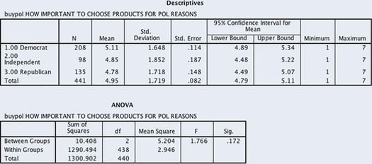
Figure 11.2 SPSS ANOVA Output: Political Party Identification and Choosing Products for Political Reasons
A Closer Look 11.2Assessing the Relationship Between Variables
Based on our five-step model of F, we’ve determined that there is a significant difference between the four demographic groups in their educational attainment. We rejected the null hypothesis and concluded that the years of education (our dependent variable) do vary by group membership (our independent variable). But can we say anything about how strong the relationship is between the variables?
The correlation ratio or eta square (η2) allows us to make a statement about the strength of the relationship or the effect size. Eta square is determined by the following:
(11.10)
η2=SSBSSTη2=SSBSST
The ratio of SSB to SST (SSB + SSW) represents the proportion of variance that is explained by the group (or independent) variable. Eta square indicates the strength of the relationship between the independent and dependent variables, ranging in value from 0 to 1.0. As eta square approaches 0, the relationship between the variables is weaker, and as eta square approaches 1, the relationship between the variables is stronger.
Based on our ANOVA example,
η2=63.0363.03+62.03=.50η2=63.0363.03+62.03=.50
We can state that 50% of the variation in educational attainment can be attributed to demographic group membership. Or we can say that 50% of the variation in the dependent variable (educational attainment) can be explained by the independent variable (group membership). So how strong is this relationship? We can base our determination of the strength on A Closer Look 10.2 from Chapter 10, the same scale that we used to assess gamma. We conclude that there is a very strong relationship between group membership and educational attainment.
LEARNING CHECK 11.4
Calculate eta square for the model presented in Figure 11.2.
READING THE RESEARCH LITERATURE: COLLEGE SATISFACTION AMONG LATINO STUDENTS
Like bivariate, t test, or chi-square analyses, ANOVA can help us understand how the categories of experience—race, age, class, and/or gender—shape our social lives. ANOVA allows us to investigate a variety of social categories by comparing the differences between them. We conclude this chapter with an example of how ANOVA is presented and interpreted in the social science literature.
Young Kim, Liz Rennick, and Marla Franco (2014)3 investigated the levels of college engagement and satisfaction among Latino undergraduate students attending highly selective colleges and universities in comparison with other racial/ethnic groups. The Latino student population is often characterized as academically unprepared for college; however, recent research has indicated that Latino students demonstrate a stronger drive to success and a higher level of academic effort compared to their peers. The 2014 research by Kim et al. is among the few studies to consider the experience of Latino students at selective colleges and universities.
Their research is based on the 2010 University of California Undergraduate Experience Survey. Kim and their colleagues limited their analyses to the outcomes of 33,415 junior and senior students. All factors were measured on a 6-point Likert-type scale: 1 = very poor to 6 = excellent. Selected results are presented in Table 11.4.4
The table presents ANOVA results for four models regarding the student satisfaction with the educational experience. The mean and standard deviation for each racial/ethnic group are reported in the table along with the obtained F ratio. The sample sizes for each racial/ethnic student group are not reported. All models are significant at the .001 level. The researchers briefly summarize their findings:
In terms of satisfaction with the educational experience, Latino students rated their satisfaction with quality of instruction and courses in the major, advising and out-of-class contact, and library support as equal to or higher than all other racial/ethnic groups. Sense of belonging and overall college satisfaction was the only area where White students reported higher levels of satisfaction than Latino students. (p. 253)5
Table 11.4 Patterns of College Experiences by Student Race/Ethnicity
|
Latino |
African American |
Asian |
White |
F | |
|
Quality of instruction and courses in the major |
M = 5.38, SD = 1.75 |
M = 5.20, SD = 1.80 |
M = 4.78, SD = 1.76 |
M = 5.37, SD = 1.77 |
225.28*** |
|
Sense of belonging and satisfaction |
M = 4.88, SD = 1.80 |
M = 4.51, SD = 1.84 |
M = 4.45, SD = 1.74 |
M = 5.12, SD = 1.81 |
287.07*** |
|
Satisfaction with advising and out of class contact |
M = 5.21, SD = 1.80 |
M = 5.16, SD = 1.87 |
M = 4.92, SD = 1.74 |
M = 5.21, SD = 1.74 |
66.26*** |
|
Satisfaction with library support |
M = 5.30, SD = 1.80 |
M = 5.23, SD = 1.85 |
M = 4.76, SD = 1.76 |
M = 5.14, SD = 1.75 |
142.00*** |
Source: Adapted from Young Kim, Liz Rennick, and Marla Franco, “Latino College Students at Highly Selective Institutions: A Comparison of Their College Experiences and Outcomes to Other Racial/Ethnic Groups,” Journal of Hispanic Higher Education 13, no. 4 (2014): 254.
*** p < .001.
They state, “We may argue that the college experiences of Latino students at highly selective research institutions are favorable and meaningful, which may contribute to development in desired educational outcomes at these types of institutions” (p. 258).
LEARNING CHECK 11.5
For the “Sense of Belonging and Satisfaction” ANOVA model, what additional information would you need to determine the F critical?
Data at Work
Kevin Hemminger: Sales Support Manager/ Graduate Program in Research Methods and Statistics

Photo courtesy of Kevin Hemminger
While working as a sales support manager for a travel management company, Kevin decided to return to school to pursue a degree in criminal justice. Although originally he intended to become a probation officer for the juvenile court system, his career trajectory went into a different direction after taking a statistics course. “Due in great part to an incredible professor who made the subject enjoyable and interesting, I decided to pursue a PhD in Research Methods and Statistics in order to teach research methods and statistics. . . . My hope is to teach on either the graduate level, or to gifted high school students preparing for college.”
Kevin has incorporated what he’s learned about methods and statistics into his sales support work. “Being a very customer-focused company in a very customer-centric field, the idea of surveying customers is critical and being able to incorporate a knowledgeable administration of surveys has been integral to my team’s success. Knowing research best practices and understanding what constitutes good, valid research has made a tremendous impact on the value of the data I provide to my leaders. My knowledge in the field has also given me a confidence level in speaking about quantitative data that I never had before. I work with enormous data sets and spreadsheets on a daily basis and understanding even the most basic concepts such as mean, median, mode, standard deviation, and variance has allowed me to lead projects and present findings in a much more intelligent way.”
He recently completed his master’s degree and is currently working on his doctorate. Kevin offers these fine words of encouragement for anyone considering data and statistical work: “If you’re thinking about pursuing a career involving statistics, my recommendation is to dive full throttle into a study or project you’re incredibly passionate about. Watching your study move from an idea, to a literature review, to a hypothesis, data collection, and then data analysis is one of the best ways to confirm your interest—and, by far, the best way to experience the power behind statistics as a discipline. If you get excited watching your data come in, and even more excited wondering [what] you’re going to do with that data, I think you’ve confirmed there is no question you’d enjoy the field! If you’re learning stats concepts and all you can think about is how you’d teach that concept to others—it’s over! You’re perfect for the field.”
Main Points
- Analysis of variance (ANOVA) procedures allows us to examine the variation in means in more than two samples. To determine whether the difference in mean scores is significant, ANOVA examines the differences between multiple samples, as well as the differences within a single sample.
- One-way ANOVA is a procedure using one dependent variable and one independent variable. The five-step hypothesis testing model is applied to one-way ANOVA.
- The test statistic for ANOVA is F. The F statistic is the ratio of between-group variance to within-group variance.
KEY TERMS
analysis of variance (ANOVA) 374
between-group sum of squares (SSB) 377
F critical 381
F obtained 381
one-way ANOVA 374
total sum of squares (SST) 377
within-group sum of squares (SSW) 377
Digital Resources
Get the tools you need to sharpen your study skills. SAGE Edge offers a robust online environment featuring an impressive array of free tools and resources. Access practice quizzes, eFlashcards, video, and multimedia at edge.sagepub.com/frankfort9e.
SPSS Demonstration [GSS18SSDS-A]
Computing Analysis of Variance Models
Social scientists have examined the association between a woman’s fertility decisions (deciding whether and/or when to have a child) and her wages, employment status, and education, along with other socioeconomic and demographic factors. Research has indicated that different social groups may have different norms and values about fertility.6
In this example, we’ll investigate the relationship between a woman’s educational attainment and the age at which her first child was born using GSS2018SSDS-A. We first analyzed this relationship in Exercise 8 of Chapter 4. Using education as the independent variable and age at which her first child was born as the dependent variable, we can assess whether there is a relationship between educational attainment and age at first childbirth.
We’ll use two variables for our analysis, the variable DEGREE (five categories of educational attainment) and AGEKDBRN (respondent’s age when her first child was born). But first, we’ll restrict our analysis to women in the GSS sample (using Data—Select Cases command. You will have to select the option “If the condition is satisfied,” then type SEX = 2 to restrict your analysis to women).
We can compute the ANOVA model by clicking on Analyze, Compare Means, then One-Way ANOVA. The opening dialog box requires that we insert AGEKDBRN in the box labeled “Dependent List” and in the box labeled “Factor” insert DEGREE.
Click on the Options button at the upper right. Click on Descriptive in the Statistics box. This will produce a table of means and standard deviations along with the ANOVA statistics. Click on Continue in the Options box, then OK in the One-Way ANOVA box.
We are interested in the F statistic and significance in the ANOVA table (Figure 11.3). Based on the output, F is 38.392 significant at the .000 level. The data reveal a positive relationship—the higher one’s educational attainment, the higher the age of first childbirth. The oldest average age at first childbirth is for women with graduate degrees (27.42 years of age), followed by women with bachelor’s degrees (26.28 years of age). The youngest group of first-time mothers is women with less than a high school diploma. On average, women with less than a high school diploma had their first child at 19.58 years of age. When compared with the age of graduate-degree first-time mothers, there is a difference of 7.84 years.
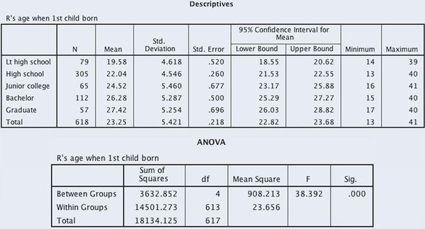
Figure 11.3
SPSS Problems [GSS18SSDS-A and B]
- S1. Let’s continue to examine the relationship between fertility decisions and education using GSS18SSDS-A. But this time, we’ll analyze the relationship for men.
- Run a Select Cases, selecting only men for the analysis.
- Compute an ANOVA model for men, using age at first-born child (AGEKDBRN) as the dependent variable and educational degree (DEGREE) as the independent variable. Based on the SPSS output, what can you conclude about the relationship between degree attainment and AGEKDBRN for men? How do these results compare with the results for women in the SPSS demonstration? Use alpha = .05.
- S2. Repeat Exercise 1b, substituting respondent’s social class (CLASS) as the independent variable in separate models for men and women. What can you conclude about the relationship between CLASS and AGEKDBRN based on an alpha of .01?
- S3. What is the ideal number of children a family should have (variable CHLDIDEL)? Use CHLDIDEL as your dependent variable and DEGREE as your independent variable. Is there a significant difference in the number of ideal children among different educational groups? (Option: You can run three sets of analyses—first, for all GSS respondents; second, an ANOVA model for women only; and finally, a model for men. Make sure to select the Descriptives option.) Evaluate your model results based on an alpha of .05.
- S4. Using GSS18SSDS-B, treat NEWS (how often do you read the newspaper) as your dependent variable and DEGREE (respondent’s educational degree) as your independent variable. Setting alpha = .05, assess the significance of both models. NEWS is coded on a 5-point scale: 1 = everyday, 2 = few times a week, 3 = once a week, 4 = less than once a week, and 5 = never.
- S5. Repeat Exercise S4, separating results by SEX. Does the relationship change when including SEX as a control variable? Explain.
Excel Demonstration [GSS18SSDS-E]
Computing Analysis of Variance Models
Although it is a bit tedious for social scientists to run an ANOVA test in Excel owing in part to the fact that we are often interested in mean differences across categorical data like race, highest degree earned, marital status, and so on with unequal sample sizes across categories, it can be done.
In this demonstration, we will use GSS18SSDS-E to examine the relationship between highest degree earned (DEGREE) and perception of the ideal number of children (CHLDIDEL). Do those with more education prefer fewer children than those with less education?
To begin our analysis, copy the DEGREE and CHLDIDEL data from the protected Data View sheet and paste it into a new Excel sheet (see Figure 11.4).
Because Excel’s ANOVA feature works with numeric data, we need to reorganize our CHLDIDEL data into five distinct columns with one column for each category (Less Than High School, High School, Junior College, Bachelor’s Degree, and Graduate Degree). To do this, we will enter Less Than High School in cell E1, High School in cell F1, and so on (see Figure 11.5). Notice that we widened the columns so the categories are clearly visible.
With all of the data in column A (from A1 to A136) selected, navigate to the Excel Data tab. Click on Sort. A “Sort Warning” window may appear. Select “Expand the selection” and then hit “Sort.” A “Sort” window will appear. Under “Column,” choose “Degree” and then hit OK. Excel will now sort all of the data by DEGREE (see Figure 11.6).
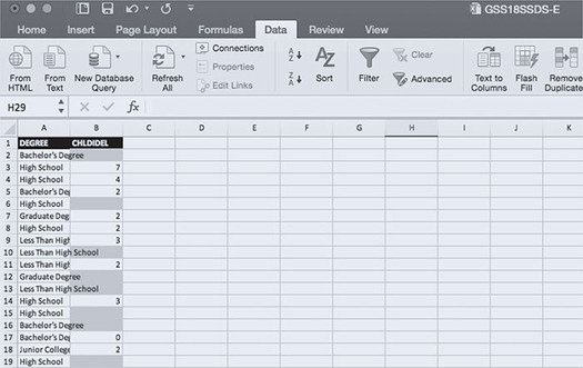
Figure 11.4
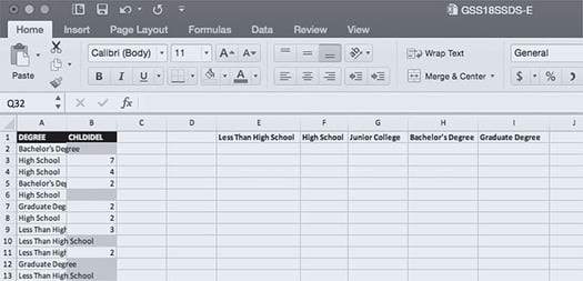
Figure 11.5

Figure 11.6
Select all of the CHLDIDEL data for respondents who have “Less Than High School” recorded for their highest degree earned—B114 to B136. On the main Excel toolbar, select Edit → Copy. Click on cell E2 (the cell directly under “Less Than High School”), and then on the main Excel toolbar, select Edit → Paste. You just successfully copied and pasted CHLDIDEL data for those who have Less Than High School. Repeat these steps for the other degree categories. For High School you will select CHLDIDEL data from B28 to B103. For Junior College, you will select CHLDIDEL data from B104 to B113. For Bachelor’s Degree, you will select CHLDIDEL data from B2 to B17. And, last, for Graduate Degree, you will select CHLDIDEL data from B18 to B27. We can now use Excel to run an ANOVA test to examine the relationship between highest degree earned and ideal number of children (see Figure 11.7).
Navigate to Excel’s Data tab. Select Data Analysis. A Data Analysis window will appear. Choose “Anova: Single Factor” and hit OK.
An “Anova: Single Factor” window will appear (see Figure 11.8). Under “Input,” click in the empty box next to “Input Range” and then select all of the CHLDIDEL data that we organized into columns by highest degree earned. In the “Input Range” box, you should see $E$1:$I$77. Next to “Grouped By,” make sure “Columns” is selected. Also make sure “Labels in first row” is selected. The default alpha is .05—you can change this if necessary. Under “Output options,” click in the empty box next to “Output Range” and select any cell in the current Excel sheet where you’d like the ANOVA results to appear. In this demonstration, we’ve chosen cell K3. Hit OK. We are now ready to interpret our findings.

Figure 11.7
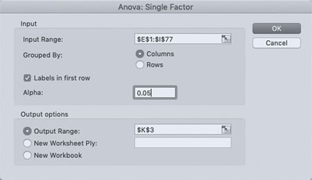
Figure 11.8
We are interested in the F statistic and significance in the ANOVA table (Figure 11.9). Based on the output, F is 2.56 with a .045 p value. If we set alpha at .05, we can conclude we are observing a significant difference in the mean number of ideal children by highest degree earned. More specifically, the data reveal a negative relationship—the higher one’s educational attainment, the fewer number of children he or she feels is ideal. Those with less than a high school diploma reported a higher ideal number of children (3.4 children) than those with a high school diploma (2.64 children), junior college (3 children), bachelor’s degree (2.14), or graduate degree (2.2).
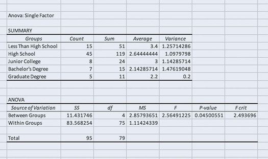
Figure 11.9
Excel Problems [GSS18SSDS-E]
- E1. Investigate whether there is a significant difference in the number of ideal children (CHLDIDEL) by marital status (MARITAL).
- Run an ANOVA test of CHLDIDEL by MARITAL.
- What is the mean ideal number of children for married respondents? Widowed? Divorced? Separated? Never married?
- What is the value of the F statistic? What p value is associated with this F statistic?
- Is there a significant difference in the ideal number of children by marital status? How do you know? Set alpha at .05.
- E2. Is there a significant difference in the age at which a respondent’s first child was born (AGEKDBRN) among different educational groups (DEGREE)?
- Run an ANOVA test of AGEKDBRN by DEGREE.
- What is the value of the F statistic? What p value is associated with this F statistic?
- Is there a significant difference in the age at which a respondent’s first child was born among different educational groups? How do you know? Set alpha at .01.
CHAPTER EXERCISES
- C1. For a random sample of 32 GSS cases, health is measured according to a 4-point scale: 1 = excellent, 2 = good, 3 = fair, and 4 = poor. Four social classes are reported here: 1 = lower, 2 = working, 3 = middle, and 4 = upper. Present the five-step model for these data, using alpha = .05.
|
Lower Class |
Working Class |
Middle Class |
Upper Class |
|
3 |
2 |
2 |
2 |
|
2 |
1 |
3 |
1 |
|
2 |
3 |
1 |
1 |
|
2 |
2 |
1 |
2 |
|
3 |
2 |
2 |
1 |
|
3 |
2 |
3 |
1 |
|
4 |
3 |
3 |
1 |
|
4 |
3 |
1 |
2 |
- C2. We take another look at health, this time examining the relationship between educational attainment and perceived quality of health care. Data for three groups are presented based on the Health Information National Trends Survey (HINTS) 2012 data set. HINTS is an annual survey measuring the use of cancer-related information for adults 18 years and older. Present the five-step model for these data, using alpha = .01. QUALITYCARE is measured on a 5-point scale: 1 = excellent, 2 = very good, 3 = good, 4 = fair, and 5 = poor. Note how a lower score indicates a higher quality of care.
Present the five-step model for these data, using alpha = .05.
|
Less Than High School |
Some College |
College Graduate |
|
1 |
2 |
1 |
|
4 |
3 |
1 |
|
2 |
2 |
1 |
|
2 |
2 |
2 |
|
3 |
4 |
1 |
|
3 |
2 |
2 |
- C3. We selected a sample of 30 International Social Science Programme respondents, noting their educational status (no degree, secondary degree, and university degree) and their level of church attendance (0 = never, 1 = infrequently, and 2 = two to three times per month or more). Is there a relationship between educational attainment and church attendance?
Complete the five-step model for these data, using alpha = .01.
|
No Degree |
Secondary Degree |
University Degree |
|
2 |
2 |
0 |
|
1 |
2 |
0 |
|
1 |
2 |
0 |
|
2 |
1 |
0 |
|
2 |
1 |
1 |
|
2 |
0 |
1 |
|
0 |
2 |
0 |
|
2 |
1 |
1 |
|
2 |
1 |
2 |
|
2 |
2 |
1 |
- C4. Based on a sample of 21 Monitoring the Future respondents, we present their racial/ethnic background and the numbers of school days missed in the past 4 weeks.
- Complete the five-step model for these data, and set alpha at .05.
- If alpha were set at .01, would your decision change? Explain.
|
White |
Black |
Hispanic |
|
4 |
1 |
4 |
|
5 |
2 |
3 |
|
3 |
2 |
5 |
|
4 |
1 |
1 |
|
4 |
3 |
5 |
|
4 |
4 |
2 |
|
6 |
3 |
2 |
- C5. We selected a sample of 14 Monitoring the Future respondents. We present their number of moving (traffic) violations in the past 12 months along with their residential area (residential area is the independent variable). Complete the five-step model for these data, using alpha = .05.
|
Small Town |
Medium-Sized City |
Large City |
|
0 |
2 |
3 |
|
0 |
3 |
4 |
|
1 |
1 |
4 |
|
2 |
1 |
3 |
|
1 |
2 |
- C6. The GSS 2014 asked respondents to identify what was important for “truly being American.” When asked “How important to have American ancestry?” answers were measured on a 4-point scale: 1 = very important, 2 = fairly important, 3 = not very important, and 4 = not important at all. We selected a sample of 20 GSS respondents and present their individual responses. Complete the five-step model for these data, using alpha = .01 to assess the significance of the model.
|
White |
Black |
Other |
|
3 |
1 |
4 |
|
2 |
2 |
2 |
|
2 |
2 |
2 |
|
2 |
2 |
2 |
|
3 |
1 |
3 |
|
4 |
1 |
2 |
|
4 |
2 |
— |
- C7. Nan Sook Park and her colleagues (2012) investigated racial/ethnic differences in predictors of self-rating health and the use of sociocultural resources. Their data are based on the Survey of Older Floridians, a statewide sample of white, African American, Cuban, and non-Cuban Hispanic seniors.
- We present ANOVA results for two sociocultural resources. Social support was measured with the question: In times of trouble, can you count on at least some of your family and friends? (1 = hardly ever, 2 = some of the time, and 3 = most of the time). Religious attendance was measured according to the following scale: 1 = never or almost never to 5 = more than once a week. Mean scores are presented for each racial/ethnic group, along with the standard deviation in parentheses. Review each measure of sociocultural resource and determine whether the null hypothesis would be rejected. Set alpha at .05 for each.
|
Racial/Ethnic Group Mean (Standard Deviation) | |||||
|
Variable |
Whites (n = 503) |
African Americans (n = 360) |
Cubans (n = 328) |
Non-Cuban Hispanics (n = 241) |
F |
|
Social support |
2.85 (0.47) |
2.75 (0.57) |
2.73 (0.60) |
2.58 (0.70) |
12.17*** |
|
Religious attendance |
2.79 (1.57) |
3.94 (1.21) |
2.74 (1.49) |
3.37 (1.43) |
56.43*** |
- Source: Nan Sook Park, Yuri Jan, Beom Lee, and David Chiriboga, “Racial/Ethnic Differences in Predictors of Self-Rated Health: Findings From the Survey of Older Floridians,” Research on Aging 35, no. 1 (2012): 207.
- *** p < .001.
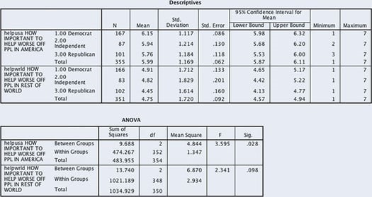
- C8. The GSS 2014 included a series of questions about what it takes to be a good citizen. Respondents were asked, to be a good citizen, how important was it “to help people in America who are worse off than yourself” (HELPUSA) and “to help people in the rest of the world who are worse off than yourself” (HELPWRLD). Answers were measured on a 7-point scale: 1 = not important at all to 7 = very important. We ran ANOVA models for each with respondent’s political party (RPartyId) as the independent variable. Set alpha at .05 to assess the significance of each model.
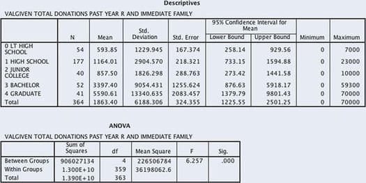
- C9. The following ANOVA model examines the relationship between DEGREE (respondent’s educational degree) and VALGIVEN (total dollar value of all donations made in the past year). Data are from the GSS 2014. Is there a significant difference in donation amount by educational degree? Set alpha at .01.
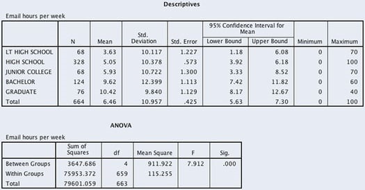
- C10. Is there a significant difference in e-mail hours per week among the same educational groups? Using data from the GSS 2018, we ran an ANOVA model using DEGREE (educational attainment) as the independent variable and EMAILHR (e-mail hours per week) as the dependent variable. Based on an alpha of .05, what do you conclude?
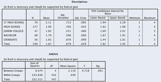
- C11. We examine the relationship between educational attainment (DEGREE) and agreement to the statement, “Scientific research is necessary and should be supported by the federal government” as measured in the GSS 2018. Responses to the scientific research statement (ADVFRONT) are measured on an ordinal scale: 1 = strongly agree, 2 = agree, 3 = neither, 4 = disagree, and 5 = strongly disagree. Does agreement vary by one’s educational degree?
- Set alpha at .01, and test the null hypothesis of equal means.
- What is the eta square for this model?
- C12. Using Monitoring the Future 2017 data, we examine whether a relationship exists between the race/ethnicity of a student and how the student rates the importance of being a community leader. IMPLDRCOMUNTY is measured on an ordinal scale: 1 = not important, 2 = somewhat important, 3 = quite important, and 4 = extra important. Analysis of variance results are presented.
- Set alpha at .05. What do you conclude about the relationship between student race/ethnicity and the importance of being a community leader?
- What is the eta square for this model?
- If alpha were set at .01, would your decision change? Explain.
- C13. In Chapter 4’s Statistics in Practice, we reviewed Myron Pope’s 2002 research on community college mentoring. Pope compared responses from four groups of minority students, measuring their perception of multilevel mentoring at their school. Student responses were based on a 5-point scale: 1 = no agreement to 5 = strong agreement. Pope’s results are presented again with an additional column of F test and significance.
- What are the degrees of freedom for the models?
- Based on an alpha of .05, assess each model. What do you conclude?
|
African American (n = 178), M (SD) |
Asian (n = 12), M (SD) |
Hispanic (n = 28), M (SD) |
Native American (n = 22), M (SD) |
Multiethnic (n = 14), M (SD) |
F Test Sig. | |
|
There are persons of color in administrative roles from whom I would seek mentoring at this institution. |
3.76 (1.10) |
3.50 (1.31) |
3.14 (1.08) |
4.09 (.68) |
4.14 (.66) |
3.508 .008 |
|
There are peer mentors who can advise me. |
3.48 (1.11) |
2.17 (1.40) |
3.14 (1.20) |
3.91 (.68) |
3.29 (1.54) |
5.245 .000 |
|
I mentor other students. |
3.30 (1.25) |
2.00 (1.21) |
3.00 (1.09) |
3.46 (1.10) |
3.29 (1.07) |
3.702 .006 |
Source:Adapted from Myron Pope, “Community College Mentoring Minority Student Perception,” Community College Review 30, no. 3 (2002): 37.
Descriptions of Images and Figures
The value of critical F on the horizontal axis is 3.13, and the value of obtained F is 6.44. The region to the right of critical F value is shaded and labeled, alpha equals 0.05.
The first table is titled, “Descriptives. Buypol How important to choose products for pol reasons.” Data from the table are as follows.
|
No data |
N |
Mean |
Standard Deviation |
Standard Error |
Lower bound 95 percent confidence interval for mean |
Upper bound 95 percent confidence interval for mean |
Minimum |
Maximum |
|
1.00 Democrat |
208 |
5.11 |
1.648 |
0.114 |
4.89 |
5.34 |
1 |
7 |
|
2.00 Independent |
98 |
4.85 |
1.852 |
0.187 |
4.48 |
5.22 |
1 |
7 |
|
3.00 Republican |
135 |
4.78 |
1.718 |
0.148 |
4.49 |
5.07 |
1 |
7 |
|
Total |
441 |
4.95 |
1.719 |
0.082 |
4.79 |
5.11 |
1 |
7 |
The second table is titled, “ANOVA. Buypol How important to choose products for pol reasons.” Data from the table are as follows.
|
No data |
Sum of squares |
df |
Mean Square |
F |
Sig |
|
Between groups |
10.408 |
2 |
5.204 |
1.766 |
0.172 |
|
Within groups |
1290.494 |
438 |
2.946 |
No data |
No data |
|
Total |
1300.902 |
440 |
No data |
No data |
No data |
The first table is titled, “Descriptives. R’s age when first child was born.” Data from the table are as follows.
|
No data |
N |
Mean |
Standard Deviation |
Standard Error |
Lower bound 95 percent confidence interval for mean |
Upper bound 95 percent confidence interval for mean |
Minimum |
Maximum |
|
Less than high school |
79 |
19.58 |
4.618 |
0.820 |
18.55 |
20.62 |
17 |
39 |
|
High school |
305 |
22.04 |
4.546 |
0.260 |
21.53 |
22.55 |
13 |
40 |
|
Junior college |
65 |
24.52 |
5.640 |
0.677 |
23.17 |
25.88 |
16 |
41 |
|
Bachelor |
112 |
26.28 |
5.287 |
0.500 |
25.29 |
27.27 |
15 |
40 |
|
Graduate |
57 |
27.42 |
5.254 |
0.696 |
26.03 |
28.82 |
17 |
40 |
|
Total |
618 |
23.52 |
5.421 |
0.218 |
22.82 |
23.68 |
13 |
41 |
The second table is titled, “ANOVA. R’s age when first child born.” Data from the table are as follows.
|
No data |
Sum of squares |
df |
Mean Square |
F |
Sig |
|
Between groups |
3632.852 |
4 |
908.213 |
38.392 |
0.000 |
|
Within groups |
14501.273 |
613 |
23.656 |
No data |
No data |
|
Total |
18134.125 |
617 |
No data |
No data |
No data |
The first row of column A is labeled Degree, and the entries in the column include Less than High School, High School, Junior College, Bachelor’s Degree, and Graduate Degree. The first row of column B is labeled CHLDIDEL, and the entries in the column include blank spaces and numbers.
The first row of column A is labeled Degree, and the entries in the column include Less than High School, High School, Junior College, Bachelor’s Degree, and Graduate Degree. The first row of column B is labeled CHLDIDEL, and the entries in the column include blank spaces and numbers. The entries in the other cells are as follows. E 1: Less than High School, F 1: High School, G 1: Junior College, H 1: Bachelor’s Degree, and I 1: Graduate Degree.
The first row of column A is labeled Degree, and the entries in the column include Less than High School, High School, Junior College, Bachelor’s Degree, and Graduate Degree. The first row of column B is labeled CHLDIDEL, and the entries in the column include blank spaces and numbers. The entries in the other cells are as follows. E 1: Less than High School, F 1: High School, G 1: Junior College, H 1: Bachelor’s Degree, and I 1: Graduate Degree.
The first row of column A is labeled Degree, and the entries in the column include Less than High School, High School, Junior College, Bachelor’s Degree, and Graduate Degree. The first row of column B is labeled CHLDIDEL. The first row of column E is labeled Less Than High School. The first row of column F is labeled High School. The first row of column G is labeled Junior College. The first row of column H is labeled Bachelor’s Degree. The first row of column I is labeled Graduate Degree. The entries in columns B, E, F, G, H, and I include blank spaces and numbers.
The dialog box consists of two sections. The first section is labeled Input, and consists of the following elements: Entry field Input Range with entry dollar sign E dollar sign 1 colon dollar sign I dollar sign 77, two radio buttons under grouped by, labeled columns and rows, and entry field Alpha with the entry 0.05. Columns is selected. A checked checkbox, Labels, is between the third and the fourth entry fields. The second section is labeled Output Options, and shows the following radio buttons: Output Range with entry dollar sign K dollar sign 3, New Worksheet Ply with empty field, and New Workbook. Output Range is selected.
The first table is titled, “Summary.” Data from the table are as follows.
|
Groups |
Count |
Sum |
Average |
Variance |
|
Less than high school |
15 |
51 |
3.4 |
1.25714286 |
|
High school |
45 |
119 |
2.64444444 |
1.0979798 |
|
Junior college |
8 |
24 |
3 |
1.14285714 |
|
Bachelor’s degree |
7 |
15 |
2.14285714 |
1.47619048 |
|
Graduate degree |
5 |
11 |
2.2 |
0.2 |
The second table is titled, “ANOVA.” Data from the table are as follows.
|
Source of variation |
SS |
df |
MS |
F |
P-value |
F crit |
|
Between groups |
11.431746 |
4 |
2.85793561 |
2.56491225 |
0.04500551 |
2.493696 |
|
Within groups |
53.568254 |
75 |
1.11424339 |
No data |
No data |
No data |
|
Total |
95 |
79 |
No data |
No data |
No data |
No data |
In both tables, the first row header is labeled, helpusa, how important to help worse off people in America.
The first table is titled, “Descriptives.” Data from the table are as follows.
|
No data |
N |
Mean |
Standard Deviation |
Standard Error |
Lower bound 95 percent confidence interval for mean |
Upper bound 95 percent confidence interval for mean |
Minimum |
Maximum |
|
America, 1.00 Democrat |
167 |
6.15 |
1.117 |
0.086 |
5.98 |
6.32 |
1 |
7 |
|
America, 2.00 Independent |
87 |
5.94 |
1.214 |
0.130 |
5.68 |
6.20 |
2 |
7 |
|
America, 3.00 Republican |
101 |
5.76 |
1.184 |
0.118 |
5.53 |
6.00 |
3 |
7 |
|
America, Total |
355 |
5.99 |
1.169 |
0.062 |
5.87 |
6.11 |
1 |
7 |
|
World, 1.00 Democrat |
166 |
4.91 |
1.712 |
0.133 |
4.65 |
5.17 |
1 |
7 |
|
World, 2.00 Independent |
83 |
4.82 |
1.829 |
0.201 |
4.42 |
5.22 |
1 |
7 |
|
World, 3.00 Republican |
102 |
4.45 |
1.614 |
0.160 |
4.13 |
4.77 |
1 |
7 |
|
World, Total |
351 |
4.75 |
1.720 |
0.092 |
4.57 |
4.94 |
1 |
7 |
The second table is titled, “ANOVA.” Data from the table are as follows.
|
No data |
Sum of squares |
df |
Mean Square |
F |
Sig |
|
America, Between groups |
9.688 |
2 |
4.844 |
3.595 |
0.028 |
|
World, Within groups |
474.267 |
352 |
1.347 |
No data |
No data |
|
America, Total |
483.955 |
354 |
No data |
No data |
No data |
|
World, Between groups |
13.740 |
2 |
6.870 |
2.341 |
0.098 |
|
World, Within groups |
1021.189 |
348 |
2.934 |
No data |
No data |
|
World, Total |
1034.929 |
350 |
No data |
No data |
No data |
The first table is titled, “Descriptives. Valgiven total donations past year R and immediate family.” Data from the table are as follows.
|
No data |
N |
Mean |
Standard Deviation |
Standard Error |
Lower bound 95 percent confidence interval for mean |
Upper bound 95 percent confidence interval for mean |
Minimum |
Maximum |
|
0 Less than high school |
54 |
593.85 |
1229.945 |
167.374 |
258.14 |
323.56 |
0 |
7000 |
|
1 High School |
177 |
1164.01 |
2904.570 |
218.321 |
733.15 |
1594.88 |
0 |
23000 |
|
2 Junior College |
40 |
857.50 |
1826.298 |
288.763 |
273.42 |
1441.58 |
0 |
10000 |
|
3 Bachelor |
52 |
3397.40 |
9054.431 |
1255.624 |
876.63 |
9801.43 |
0 |
70000 |
|
4 Graduate |
41 |
5590.61 |
13340.635 |
2083.457 |
1379.79 |
9801.43 |
0 |
70000 |
|
Total |
364 |
1863.40 |
6188.306 |
324.355 |
1225.55 |
2501.25 |
0 |
70000 |
The second table is titled, “ANOVA. Valgiven total donations past year R and immediate family.” Data from the table are as follows.
|
No data |
Sum of squares |
df |
Mean Square |
F |
Sig |
|
Between groups |
906027134 |
4 |
226506784 |
6.257 |
0.000 |
|
Within groups |
1.300 E positive 10 |
359 |
36198062.6 |
No data |
No data |
|
Total |
1.390 E positive 10 |
363 |
No data |
No data |
No data |
The first table is titled, “Descriptives. Email hours per week.” Data from the table are as follows.
|
No data |
N |
Mean |
Standard Deviation |
Standard Error |
Lower bound 95 percent confidence interval for mean |
Upper bound 95 percent confidence interval for mean |
Minimum |
Maximum |
|
Less than high school |
68 |
3.63 |
10.117 |
1.227 |
1.18 |
6.08 |
0 |
70 |
|
High School |
328 |
5.05 |
10.378 |
0.573 |
3.92 |
6.18 |
0 |
100 |
|
Junior College |
68 |
5.93 |
10.722 |
1.300 |
3.33 |
8.52 |
0 |
70 |
|
Bachelor |
124 |
9.62 |
12.399 |
1.113 |
7.42 |
11.82 |
0 |
60 |
|
Graduate |
76 |
10.42 |
9.840 |
1.129 |
8.17 |
12.67 |
0 |
40 |
|
Total |
664 |
6.46 |
10.957 |
0.425 |
5.63 |
7.30 |
0 |
100 |
The second table is titled, “ANOVA. Email hours per week.” Data from the table are as follows.
|
No data |
Sum of squares |
df |
Mean Square |
F |
Sig |
|
Between groups |
3647.686 |
4 |
911.922 |
7.912 |
0.000 |
|
Within groups |
75953.372 |
659 |
115.255 |
No data |
No data |
|
Total |
79601.059 |
663 |
No data |
No data |
No data |
The first table is titled, “Descriptives. Sci Rsch is necessary and should be supported by federal government.” Data from the table are as follows.
|
No data |
N |
Mean |
Standard Deviation |
Standard Error |
Lower bound 95 percent confidence interval for mean |
Upper bound 95 percent confidence interval for mean |
Minimum |
Maximum |
|
Less than high school |
70 |
2.11 |
0.713 |
0.085 |
1.94 |
2.28 |
1 |
4 |
|
High School |
277 |
1.90 |
0.700 |
0.042 |
1.82 |
1.98 |
1 |
4 |
|
Junior College |
47 |
1.85 |
0.551 |
0.080 |
1.69 |
2.01 |
1 |
3 |
|
Bachelor |
98 |
1.79 |
0.596 |
0.060 |
167 |
1.91 |
1 |
4 |
|
Graduate |
56 |
1.63 |
0.676 |
0.090 |
1.44 |
1.81 |
1 |
3 |
|
Total |
548 |
1.87 |
0.679 |
0.029 |
1.82 |
1.93 |
1 |
4 |
The second table is titled, “ANOVA. Sci Rsch is necessary and should be supported by federal government.” Data from the table are as follows.
|
No data |
Sum of squares |
df |
Mean Square |
F |
Sig |
|
Between groups |
8.474 |
4 |
2.119 |
4.718 |
0.001 |
|
Within groups |
243.838 |
543 |
0.449 |
No data |
No data |
|
Total |
252.312 |
547 |
No data |
No data |
No data |
The first table is titled, “Descriptives. 171A007H:IMP LDR COMUNTY.” Data from the table are as follows.
|
No data |
N |
Mean |
Standard Deviation |
Standard Error |
Lower bound 95 percent confidence interval for mean |
Upper bound 95 percent confidence interval for mean |
Minimum |
Maximum |
|
Black 1 |
276 |
2..91 |
0.996 |
0.060 |
2.79 |
3.03 |
1 |
4 |
|
White 2 |
1041 |
2.51 |
0.969 |
0.030 |
2.45 |
2.57 |
1 |
4 |
|
Hispanic 3 |
380 |
2.53 |
1.005 |
0.052 |
2.43 |
2.64 |
1 |
4 |
|
Total |
1697 |
2.58 |
0.991 |
0.024 |
2.53 |
2.63 |
1 |
4 |
The second table is titled, “ANOVA. 171A007H:IMP LDR COMUNTY.” Data from the table are as follows.
|
No data |
Sum of squares |
df |
Mean Square |
F |
Sig |
|
Between groups |
35.836 |
2 |
17.918 |
18.605 |
0.000 |
|
Within groups |
1631.435 |
1694 |
0.963 |
No data |
No data |
|
Total |
1667.270 |
1696 |
No data |
No data |
No data |
Resources
- 24 x 7 Availability.
- Trained and Certified Experts.
- Deadline Guaranteed.
- Plagiarism Free.
- Privacy Guaranteed.
- Free download.
- Online help for all project.
- Homework Help Services

