Evaluating Household Data Assessment 1
Assessment 1 - Evaluating Household Data
Data Set: Household data
Data set :. This includes information about 2000 households across the following variables.
These are the different variables we have to consider.
There are 15 different variables we will consider for the study.
Tasks for Analysis of Data Set
Task 1
- Random sample of size 250.
We have used here random number generation method. Due to this method bias will get reduced and we get better results.
A random number generator (RNG) is a device that generates a sequence of numbers or symbols that cannot be reasonably predicted better than by a random chance.
We have used Uniform random number generation method. So the random variable will be lies between 0 and 1.
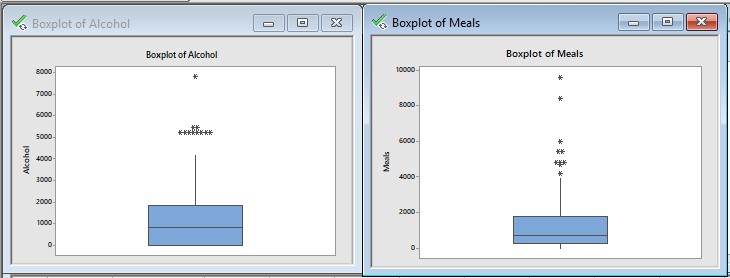
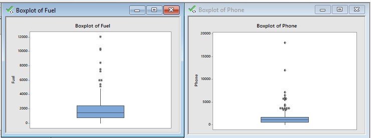
- Descriptive statistics and boxplot of Alcohol, Meals, Fuel and Phone.
Now we have to find descriptive statistics of each variable in the data set. Also we have to draw boxplot of each variable.
The descriptive statistics are in excel file (sheet 3).
Box plot of Alcohol, Meals, Fuel and Phone :


- Interpretation of descriptive statistics and boxplot :
From descriptive statistics we can say that,
Average annual expenditures on alcohol in AUD is higher than that of meals, fuel and phone.
"Skewness assesses the extent to which a variable’s distribution is symmetrical.
Kurtosis is a measure of whether the distribution is too peaked (a very narrow distribution with most of the responses in the center).
We can see that skewness coefficient for all the four variables is greator than 0 so distribution is positively skewed.
For Alcohol kurtosis = 2.86 < 3 the distribution is platykurtic.
For meals, fuel and phone the kurtosis coefficients are 8.31, 8.43 and 43.57 respectively which are greator than 3 so the distribution for all three is leptokurtic.
Interpretation of boxplot :
From all the boxplots we can see that some points are outside the boxplot. They seems to be outlier.
In all the four variables there are outliers present in the sample implies population is also contains outliers.
Task 2
- Frequency distribution of expenditure of Utilities
Here interest of variable is Utilities.
We have to construct frequency distribution of the expenditures on Utilities.
We have to construct frequency distribution having 11 classes.
The classes are 0-300, 300-600, ............., 2700-3000, More than 3000.
First arrange the data of Utilities in ascending order.
Now we have to find frequency for each class.
Frequency of the class is the number of observations in the particular class.
Class 0-300 contains observations between 0 and including 299.
Class 300-600 contains observations between 300 and including 599 and so on.
In this way we will complete frequency distribution.
The frequency distribution of Utility expenditure is,
|
Classes |
frequency |
|
0-300 |
16 |
|
300-600 |
33 |
|
600-900 |
51 |
|
900-1200 |
36 |
|
1200-1500 |
38 |
|
1500-1800 |
30 |
|
1800-2100 |
20 |
|
2100-2400 |
10 |
|
2400-2700 |
5 |
|
2700-3000 |
1 |
|
More than 3000 |
10 |
|
Totals |
250 |
- Different percenatges of households who spend on Utilities
- at the most $900 per annum
To find P(Percentage of households who spend on Utilities ≤ $900).
= P(0-300 or 300-600 or 600-900)
= P(0-300 class) + P(300-600 class) + P(600-900 class)
16/250 +33/250 + 51/250 = 100/250 =0.4 = 0.4*100 = 40%
- between $1500 and $2700 per annum, and
To find P(Percentage of households who spend on Utilities between $1500 and $2700).
= P(1500-1800 or 1800-2100 or 2100-2400 or 2400-2700)
= P(1500-1800) + P(1800-2100) + P(2100-2400) + P(2400-2700)
30/250 + 20/250 + 10/250 + 5/250 = 65/250 = 0.26*100 = 26%
- more than $3000 per annum.
To find P(Percentage of households who spend on Utilities more than $3000).
= P(more than 3000)
= 10/250 =0.04 = 0.04*100 = 4%
Task 3
- Top 5% value and the bottom 5% value of the household’s annual after-tax income.
Here our interest of variable is households annual after tax income (AtaxInc).
Let X be the random variable that value of the households annual after tax income.
Here we need to find descriptive statistics for AtaxInc.
From the descriptive statistics :
X ~ N(µ= 60113.04 , σ = 41293.33)
Top 5% we can write symbolically as,
P(X > x) = 5% = 0.05
1 – P(X≤ x) = 0.05
P(X ≤ x) = 1 – 0.05
P(X ≤ x) = 0.95
Now by using EXCEL,
Z = 1.645
Now we can find x by using formula,
X = µ+ z*σ = 60113.04 + 1.645*41293.33 = $128034.5
Thus, your AtaxInc expenditure needs to be $128034.5 or higher .
So 5% of the sample has a expenditure higher than $128034.5
Bottom 5% we can write symbolically as,
P(X < x) = 5% = 0.05
Z = -1.645
X = 60113.04 + 1.645*41293.33 = $-7808.45
Thus, your AtaxInc expenditure needs to be $128034.5 or less .
So 5% of the sample has a expenditure lower than $-7808.45
- Type of variable Ownhouse and probability distribution of Ownhouse
Here interest of variable is Ownhouse.
It contains two numbers 1 and 0.
1 : if a household owns a house
0 : if a household doesn’t owns a house
- Is this a quantitative or a qualitative variable?
This is qualitative variable because yes or no type data is present for Ownhouse.
(ii) What would be the probability distribution of this random variable if we choose randomly (a) Only 1 household? (b) 250 households? Provide any relevant condition(s) to justify your answer.
Let X be a random variable such that X = Number of households who own a house.
It will take two values 1 and 0.
Now we have to find probability for each outcomes.
|
X |
f |
P |
|
0 |
73 |
0.292 |
|
1 |
177 |
0.708 |
|
250 |
1 |
Probability distribution of X is,
|
x |
0 |
1 |
total |
|
p |
0.292 |
0.705 |
1 |
P(only 1 household) = 1/250 = 0.004
P(250 households) = 250/250 = 1
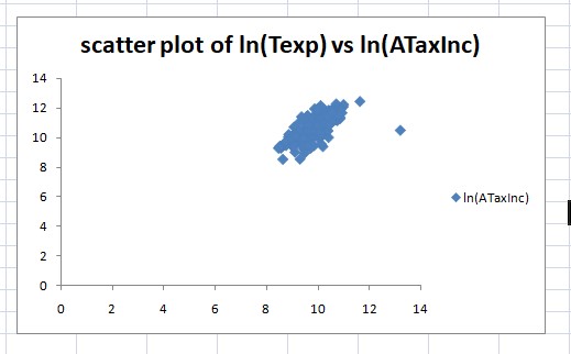
- Scatter plot of ln (Texp) Vs ln(ATaxInc) and type of correlation
Dependent variable y = ln (Texp)
Independent variable x = ln(ATaxInc)
This is the problem of simple linear regression.
By using excel we get following scatter plot.

Correlation coefficient (r) = 0.7145
Correlation coefficient have positive sign so there is positive relationship between two variables.
From the scatter plot we can say that there is positive relationship between natural logarithm of Texp and natural logarithm of ATaxInc.
Task 4
- Contingency table of gender and level of education
Here our interest of variable is gender and the level of education.
Gender has two levels male and female.
And level of education (Highest degree) has primary, secondary, intermediate, bachelors and master.
Now we have to complete contingency table of the data.
|
Highest degree | ||||||
|
Gender |
P |
S |
I |
B |
M |
total |
|
Male |
25 |
34 |
23 |
23 |
33 |
138 |
|
Female |
24 |
25 |
20 |
26 |
17 |
112 |
|
total |
49 |
59 |
43 |
49 |
50 |
250 |
- Probability of male and level of education is intermediate
To find P(male and I)
P(maleandI)= numberofhouseholdsaremaleandlevelofeducationisI/samplesize = 23/250
P(male and I) = 0.092
- Probability of female and level of education is Bachelor
To find P(female and B).
P(femaleandB) = numberofhouseholdsarefemaleandlevelofeducationisB/samplesize = 26/250
P(female and B) = 0.1040
- Proportion of secondary level of education and male
To find P(S and male).
P(Sandmale) = numberofhouseholdswhoareSandmale/samplesize = 34/250 = 0.1360
- Independence of female and level of education is Master degree.
The events are said to be independent iff
P(female * Master degree) = P(female) * P(Master degree)
17/250 = 112/250 * 50/250
17/250 56/625
0.0680 ≠ 0.0896
The events "gender of household head is female" and "having the Master Degree" dependent events.
Buy Title Answers Online
Talk to our expert to get the help with Title to complete your assessment on time and boost your grades now
The main aim/motive of the management assignment help services is to get connect with a greater number of students, and effectively help, and support them in getting completing their assignments the students also get find this a wonderful opportunity where they could effectively learn more about their topics, as the experts also have the best team members with them in which all the members effectively support each other to get complete their diploma assignments. They complete the assessments of the students in an appropriate manner and deliver them back to the students before the due date of the assignment so that the students could timely submit this, and can score higher marks. The experts of the assignment help services at urgenthomework.com are so much skilled, capable, talented, and experienced in their field of programming homework help writing assignments, so, for this, they can effectively write the best economics assignment help services.
Get Online Support for Title Assignment Help Online
Resources
- 24 x 7 Availability.
- Trained and Certified Experts.
- Deadline Guaranteed.
- Plagiarism Free.
- Privacy Guaranteed.
- Free download.
- Online help for all project.
- Homework Help Services
Testimonials
Urgenthomework helped me with finance homework problems and taught math portion of my course as well. Initially, I used a tutor that taught me math course I felt that as if I was not getting the help I needed. With the help of Urgenthomework, I got precisely where I was weak: Sheryl. Read More

