Sample Assignment on Newton's law of cooling
Mathematical model of Newton's law of cooling and experimental verification
Introduction
With the time a hot object cools down and it temperature slowly goes down till it reaches the surrounding temperature. Similarly a cold object temperature rises to the surrounding temperature with the time. In both cases object exchanges its heat with the surrounding to reach the final temperature or so called equilibrium temperate. Further we observer that more the difference in the temperature between the surrounding and the objects faster is the heat exchange under the similar condition of the other parameters.
Sir Newtown’ proposed a law called “Newton’s Law of cooling” for cooling of objects. This law states that the rate of change of the temperature of an object is proportional to the temperature difference between object’s temperature and the ambient temperature that is surroundings temperature of the objects. Such behavior has been observed many times in laboratory experiments and it is also verified, Hence Newton’s Law of cooling widely accepted. We know that object can transfer the heat to its surrounding by any of the three method of heat exchange not only due to conduction and convection but also due to radiation. The latter does not vary linearly with temperature difference, which leads to deviations from Newton's law.

The Mathematical Model
Newtown’s law of cooling - The rate of temperature change of a substance is proportional to the difference between its temperature and the ambient room temperature.
Mathematically it can be rewritten as
dT/dt = k(T - Ta)
Where T(t ) = Temperature of the object at any time t.
Ta = Ambient temperature.
T(0) = Initial Temperature of the object
K = Constant of proportionality that depends
on the nature of object and surrounding
Solving this differential equation we get and using the initial condition that temperature of objects and ambient temperature we get the equation as follows that is in the most general form.
T(t) = Ta + (To - Ta)ekt
From this equation we can drive the linear form of the plot and final formula would be
kt = in

The experiment
| Equipment | Quantity | Purpose |
| Styrofoam Cup | 1 | Hot was container |
| Hot water | NA | Experimental fluid |
| Temperature probe | 1 | To measure the temperature |
| Stop watch | 1 | For measurement time |
| Microwave | 1 | T o rise the water temperature |
Aim: Our aim is to verify that under our experimental condition that is mentioned in the above table if Newtown’s law of cooling is applicable.
Procedure: A cup of hot water at 194 degree Centigrade was taken in the Styrofoam cup with the decision based upon the availability of the cup. Putting the temperature probe in the water half dipped and then we allowed the water to cool down and we measure the temperature as following.
Observation table
| Time(min) | Temp(F) |
| O | 194 |
| 15 | 183 |
| 30 | 162 |
| 45 | 144 |
| 60 | 132 |
| 75 | 122 |
| 90 | 115 |
| 105 | 109 |
| 120 | 103 |
| 135 | 99 |
| 150 | 97 |
| 165 | 94 |
| 180 | 90 |
Experimental condition:
Initial water temperature = 194 F
Final water temperature = 90 F
Room temperature = 75 F
Number of observation point= 15
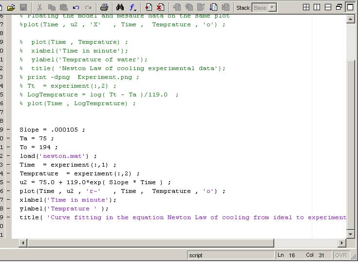
The MatLab Analysis
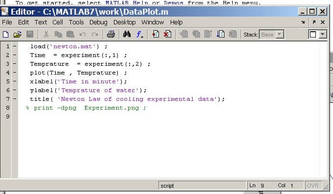
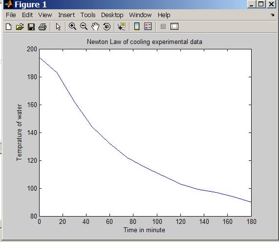
From the derivation we know that transformed equation for linear plot can be written as

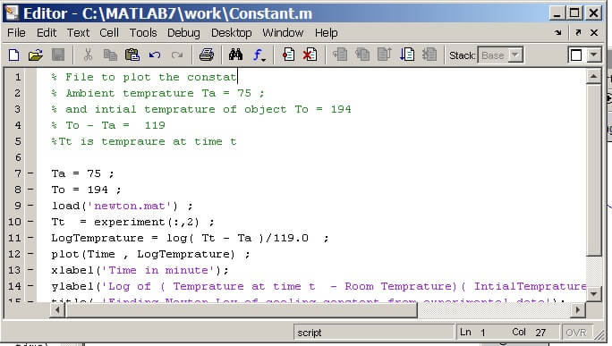
The Model
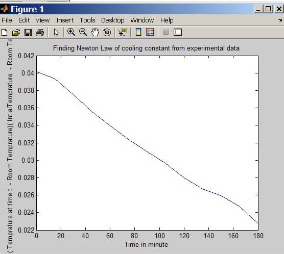
From the plot slope = Delta Y / Delta X = 0.0119 / 113 = 1.05 x 10⁻⁴
Conclusion
We see that under the laboratory condition Newton’s law of cooling holds. However various plots show the deviation from ideal behavior that is due to experiment condition and measurement errors. Accuracy of the experiment can be increase by removing the source of various avoidable and more precise time sampling
References
http://www.nsa.gov/academia/_files/collected_learning/high_school/calculus/newtons_law.pdf
http://archives.math.utk.edu/ICTCM/VOL07/C023/paper.pdf
http://www.instruction.greenriver.edu/projecttime/documents/aim/newtons_law_of_cooling-computer.pdf
http://www.instruction.greenriver.edu/projecttime/documents/aim/newtons_law_cooling_ez.pdf

